| Information |  | |
Derechos | Equipo Nizkor
| ||
| Information | | |
Derechos | Equipo Nizkor
| ||
13Nov13
Poverty in the United States: 2012
Contents
The U.S. "Official" Definition of Poverty
Racial and Ethnic Minorities
Nativity and Citizenship Status
Children
Adults with Low Education, Unemployment, or Disability
The AgedReceipt of Need-Tested Assistance Among the Poor
Poverty in Metropolitan and Nonmetropolitan Areas, Center Cities, and Suburbs
Poverty by Region
State Poverty Rates
Change in State Poverty Rates: 2002-2012
Poverty Rates by Metropolitan Area
Congressional District Poverty Estimates
"Neighborhood" Poverty--Poverty Areas and Areas of Concentrated and Extreme PovertyThe Research Supplemental Poverty Measure
Poverty Thresholds
SPM Poverty Thresholds
Resources and Expenses Included in the SPM
Poverty Estimates Under the Research SPM Compared to the "Official" MeasurePoverty by Age
Discussion
Poverty by Type of Economic Unit
Poverty by Region
Poverty by Residence
Poverty by State
Marginal Effects of Counting Specified Resources and Expenses on Poverty Under the SPM
Distribution of the Population by Ratio of Income/Resources Relative to PovertyFigures
Figure 1. Trend in Poverty Rate and Number of Poor Persons: 1959-2012, and Unemployment Rate from January 1959 through August 2013
Figure 2. U.S. Poverty Rates by Age Group, 1959-2012
Figure 3. Child Poverty Rates by Family Living Arrangement, Race and Hispanic Origin, 2012
Figure 4. Composition of Children, by Family Type, Race and Hispanic Origin, 2012
Figure 5. Percentage of People in Poverty in the Past 12 Months by State and Puerto Rico: 2012
Figure 6. Poverty Rates for the 50 States and the District of Columbia: 2012 American Community Survey (ACS) Data
Figure 7. Distribution of Poor People by Race and Hispanic Origin, by Level of Neighborhood (Census Tract) Poverty, 2006-2010
Figure 8. Poverty Thresholds Under the "Official" Measure and the Research Supplemental Poverty Measure for Units with Two Adults and Two Children: 2012
Figure 9. Poverty Rates Under the "Official"* and Research Supplemental Poverty Measures, by Age: 2012
Figure 10. Poverty Rates Under the "Official"* and Research Supplemental Poverty Measures, by Type of Economic Unit: 2012
Figure 11. Poverty Rates Under the "Official"* and Research Supplemental Poverty Measures, by Region: 2012
Figure 12. Poverty Rates Under the "Official"* and Research Supplemental Poverty Measures, by Residence: 2012
Figure 13. Difference in Poverty Rates by State Using the "Official"* Measure and the SPM: Three-Year Average 2010-2012
Figure 14. Poverty Rates by State Using the "Official"* Measure and the SPM: Three-Year Average 2010-2012
Figure 15. Poverty Rates by State Using the "Official"* Measure and the SPM: Three-Year Average 2010-2012
Figure 16. Percentage Point Change in Poverty Rates Attributable to Selected Income and Expenditure Elements Under the Research Supplemental Poverty Measure, by Age Group: 2012
Figure 17. Distribution of the Population by Income/Resources to Poverty Ratios Under the "Official"* and Research Supplemental Poverty Measures, by Age Group: 2012Tables
Table 1. Poverty Rates for the 50 States and the District of Columbia, 2002 to 2012 Estimates from the American Community Survey (ACS)
Table 2. Large Metropolitan Areas Among Those with the Lowest Poverty Rates: 2012
Table 3. Large Metropolitan Areas Among Those with the Highest Poverty Rates: 2012
Table 4. Smaller Metropolitan Areas Among Those with the Lowest Poverty Rates: 2012
Table 5. Smaller Metropolitan Areas Among Those with the Highest Poverty Rates: 2012
Table 6. Poverty Measure Concepts Under "Official" and Supplemental Measures
Table A-1. Poverty Rates (Percent Poor) for Selected Groups, 1959-2012
Table B-1. Metropolitan Area Poverty: 2012
Table C-1. Poverty by Congressional District: 2012Appendixes
Appendix A. U.S. Poverty Statistics: 1959-2012
Appendix B. Metropolitan Area Poverty Estimates
Appendix C. Poverty Estimates by Congressional District
Summary
In 2012, 46.5 million people were counted as poor in the United States--the number, statistically unchanged over the past three years, is the largest recorded in the measure's 54-year history. The poverty rate, or percent of the population considered poor under the official definition, was reported at 15.0% in 2012, a level statistically unchanged from the two previous years. The 2012 poverty rate of 15.0% is well above its most recent pre-recession low of 12.3% (2006) and remains at a level not last seen since 1993. Poverty in the United States increased markedly from 2007 through 2010, in tandem with the economic recession (officially marked as running from December 2007 to June 2009). Little if any improvement in the level of "official" U.S. poverty has been seen since the recession's official end, with the poverty rate remaining at about 15% for the past three years. Some analysts expect U.S. poverty to remain above pre-recession levels through much, if not most, of the remainder of the decade, given the slow pace of economic recovery. The pre-recession poverty rate of 12.3% in 2006 was well above the 2000 rate of 11.3%, which marked an historical low (a rate statistically tied with the previous historical low of 11.1% in 1973).
The incidence of poverty varies widely across the population according to age, education, labor force attachment, family living arrangements, and area of residence, among other factors. Under the official poverty definition, an average family of four was considered poor in 2012 if its pretax cash income for the year was below $23,492.
The measure of poverty currently in use was developed some 50 years ago, and was adopted as the "official" U.S. statistical measure of poverty in 1969. Except for minor technical changes, and adjustments for price changes in the economy, the "poverty line" (i.e., the income thresholds by which families or individuals with incomes that fall below are deemed to be poor) is the same as that developed nearly a half century ago, reflecting a notion of economic need based on living standards that prevailed in the mid-1950s.
Moreover, poverty as it is currently measured only counts families' and individuals' pre-tax money income against the poverty line in determining whether or not they are poor. In-kind benefits, such as benefits under the Supplemental Nutrition Assistance Program (SNAP, formerly named the Food Stamp program) and housing assistance are not accounted for under the "official" poverty definition, nor are the effects of taxes or tax credits, such as the Earned Income Tax Credit (EITC) or Child Tax Credit (CTC). In this sense, the "official" measure fails to capture the effects of a variety of programs and policies specifically designed to address income poverty.
A congressionally commissioned study conducted by a National Academy of Sciences (NAS) panel of experts recommended, some 19 years ago, that a new U.S. poverty measure be developed, offering a number of specific recommendations. The Census Bureau, in partnership with the Bureau of Labor Statistics (BLS), has developed a Supplemental Poverty Measure (SPM) designed to implement many of the NAS panel recommendations. The SPM is to be considered a "research" measure, to supplement the "official" poverty measure. Guided by new research, the Census Bureau and BLS intend to improve the SPM over time. The "official" statistical poverty measure will continue to be used by programs that use it as the basis for allocating funds under formula and matching grant programs. The Department of Health and Human Services (HHS) will continue to issue poverty income guidelines derived from "official" Census Bureau poverty thresholds. HHS poverty guidelines are used in determining individual and family income eligibility under a number of federal and state programs. Estimates from the SPM differ from the "official" poverty measure and are presented in a final section of this report.
Trends in Poverty |1|
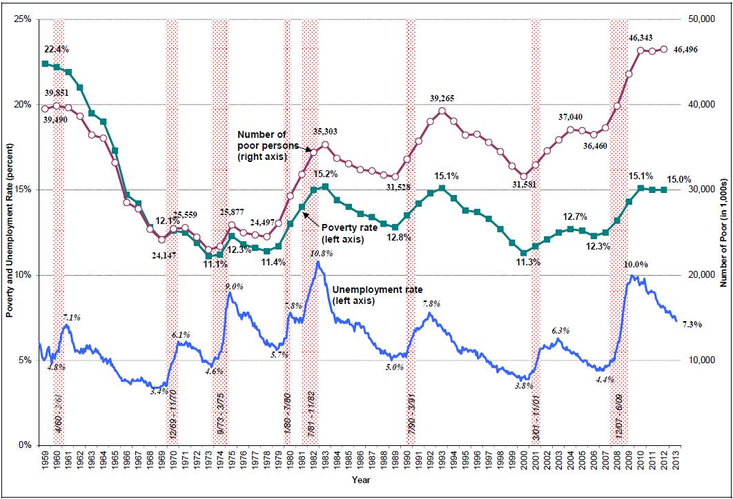
In 2012, the U.S. poverty rate was 15.0%--46.5 million persons were estimated as having income below the official poverty line. Neither the poverty rate nor the number of persons counted as poor in 2012 differed statistically from 2011 or 2010. In 2012, an estimated 10.0 million more people were poor than in 2006 and the poverty rate (15.0%) was 22% above that of 2006 (12.3%). The 46.5 million persons counted as poor in 2012 is the largest number counted in the measure's recorded history, which goes back as far as 1959, and the 2012 poverty rate of 15.0% is the highest seen since 1993. (See Figure 1.)
The increase in poverty since 2006 reflects the effects of the economic recession that began in December 2007. |2| The level of poverty tends to follow the economic cycle quite closely, tending to rise when the economy is faltering and fall when the economy is in sustained growth. This most recent recession, which officially ended in June 2009, was the longest recorded (18 months) in the post-World War II period. Even as the economy recovers, poverty is expected to remain high, as poverty rates generally do not begin to fall until economic expansion is well underway. Given the depth and duration of the recession, and the projected slow recovery, it will likely take several years or more before poverty rates recede to their 2006 pre-recession level.
The poverty rate increased markedly over the past decade, in part a response to two economic recessions. A strong economy during most of the 1990s is generally credited with the declines in poverty that occurred over the latter half of that decade, resulting in a record-tying, historical low poverty rate of 11.3% in 2000 (a rate statistically tied with the previous lowest recorded rate of 11.1% in 1973). The poverty rate increased each year from 2001 through 2004, a trend generally attributed to economic recession (March 2001 to November 2001), and failed to recede appreciably before the onset of the December 2007 recession. Over the course of the most recent recession, the unemployment rate increased from 4.9% (January 2008) to 7.2% (December 2008), and continued to rise over most of 2009, peaking at 10.1% in October. From December 2009 to December 2010, the unemployment rate fell 0.5%, from 9.9% to 9.4%, but the poverty rate in 2010 increased over 2009. The unemployment rate fell 0.9%, from 9.4% to 8.5% from December 2010 to December 2011, and by December 2012 by an additional 0.7%, to 7.8%, but the poverty rate in 2012 (15.0%) has remained at recent peak levels for three years running.
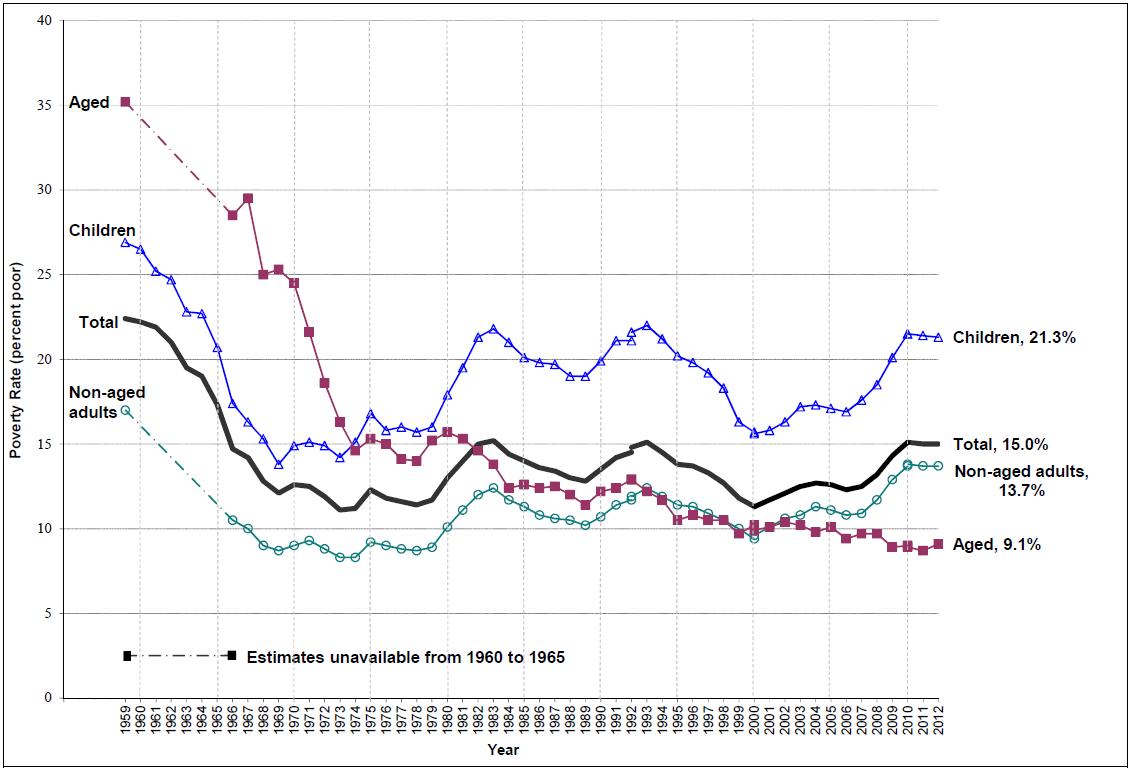
The recession especially affected non-aged adults (persons age 18 to 64) and children. (See Figure 2.) The poverty rate of non-aged adults reached 13.8% in 2010, the highest it has been since the early 1960s. |3| In 2012 and 2011, the non-aged poverty rate of 13.7% was statistically no different than in 2010. The poverty rate for non-aged adults will need to fall to 10.8% to reach its 2006 pre-recession level.
In 2012, over one in five children (21.3%) were poor, a rate statistically unchanged from the two prior years, but significantly above its 2006 pre-recession low, at which time about one in six children (16.9%) were counted as poor. Child poverty appears to be especially sensitive to economic cycles, as it often takes two working parents to support a family, and a loss of work by one may put the family at risk of falling into poverty. |4| Moreover, one-third of all children in the country live with only one parent, making them even more prone to falling into poverty when the economy falters.
In 2012, the aged poverty rate (9.1%) was statistically tied with most recent prior years, and in spite of the recession, remains at an historic low level. The longer-term secular trend in poverty has been affected by changes in household and family composition and by government income security and transfer programs. In 1959, over one-third (35.2%) of persons age 65 and over were poor, a rate well above that of children (26.9%). Social Security, in combination with a maturing pension system, has helped greatly to reduce the incidence of poverty among the aged over the years, and as recent evidence seems to show, it has helped protect them during the economic downturn.
The U.S. "Official" Definition of Poverty |5|
The Census Bureau's poverty thresholds form the basis for statistical estimates of poverty in the United States. |6| The thresholds reflect crude estimates of the amount of money individuals or families, of various size and composition, need per year to purchase a basket of goods and services deemed as "minimally adequate," according to the living standards of the early 1960s. The thresholds are updated each year for changes in consumer prices. In 2012, for example, the average poverty threshold for an individual living alone was $11,720; for a two-person family, $14,937; and for a family of four, $23,492. |7|
The current official U.S. poverty measure was developed in the early 1960s using data available at the time. It was based on the concept of a minimal standard of food consumption, derived from research that used data from the U.S. Department of Agriculture's (USDA's) 1955 Food Consumption Survey. That research showed that the average U.S. family spent one-third of its pre-tax income on food. A standard of food adequacy was set by pricing out the USDA's Economy Food Plan--a bare-bones plan designed to provide a healthy diet for a temporary period when funds are low. An overall poverty income level was then set by multiplying the food plan by three, to correspond to the findings from the 1955 USDA Survey that an average family spent one-third of its pre-tax income on food and two-thirds on everything else.
The "official" U.S. poverty measure |8| has changed little since it was originally adopted in 1969, with the exception of annual adjustments for overall price changes in the economy, as measured by the Consumer Price Index for all Urban Consumers (CPI-U). Thus, the poverty line reflects a measure of economic need based on living standards that prevailed in the mid-1950s. It is often characterized as an "absolute" poverty measure, in that it is not adjusted to reflect changes in needs associated with improved standards of living that have occurred over the decades since the measure was first developed. If the same basic methodology developed in the early 1960s was applied today, the poverty thresholds would be over three times higher than the current thresholds. |9|
Persons are considered poor, for statistical purposes, if their family's countable money income is below its corresponding poverty threshold. Annual poverty estimates are based on a Census Bureau household survey (Annual Social and Economic Supplement to the Current Population Survey, CPS/ASEC, conducted February through April). The official definition of poverty counts most sources of money income received by families during the prior year (e.g., earnings, social security, pensions, cash public assistance, interest and dividends, alimony, and child support, among others). For purposes of officially counting the poor, noncash benefits (such as the value of Medicare and Medicaid, public housing, or employer provided health care) and "near cash" benefits (e.g., food stamps, renamed Supplemental Assistance Nutrition (SNAP) benefits beginning in FY2009) are not counted as income, nor are tax payments subtracted from income, nor are tax credits added (e.g., Earned Income Tax Credit (EITC)). Many believe that these and other benefits should be included in a poverty measure so as to better reflect the effects of government programs on poverty.
The Census Bureau, in partnership with the Bureau of Labor Statistics (BLS), has recently released a Supplemental Poverty Measure (SPM), designed to address many of the perceived flaws of the "official" measure. The SPM is discussed in a separate section at the end this report (see "The Research Supplemental Poverty Measure").
Figure 1. Trend in Poverty Rate and Number of Poor Persons: 1959-2012, and Unemployment Rate from January 1959 through August 2013
(recessionary periods marked in red)
Source: Prepared by the Congressional Research Service (CRS) using U.S. Census Bureau, "Income, Poverty, and Health Insurance Coverage in the United States: 2012," Table B-1, Current Population Report P60-245, September 2013 available on the Internet at http://www.census.gov/prod/2013pubs/p60-245.pdf. Unemployment rates are available on the Internet at http://www.bls.gov/cps/. Recessionary periods defined by National Bureau of Economic Research Business Cycle Dating Committee: http://www.nber.org/cycles/main.html.
Figure 2. U.S. Poverty Rates by Age Group, 1959-2012
Source: Prepared by the Congressional Research Service using U.S. Census Bureau, "Income, Poverty, and Health Insurance Coverage in the United States: 2012," Tables B-1 and B-2, Current Population Report P60-245, September 2013, available on the Internet at http://www.census.gov/prod/20l3pubs/p60-245.pdf.
Even during periods of general prosperity, poverty is concentrated among certain groups and in certain areas. Minorities; women and children; the very old; the unemployed; and those with low levels of educational attainment, low skills, or disability, among others, are especially prone to poverty.
Racial and Ethnic Minorities |10|
The incidence of poverty among African Americans and Hispanics exceeds that of whites by several times. In 2012, 27.2% of blacks (10.9 million) and 25.6% of Hispanics (13.6 million) had incomes below poverty, compared to 9.7% of non-Hispanic whites (18.9 million) and 11.7% of Asians (1.9 million). Although blacks represent only 12.9% of the total population, they make up 23.5% of the poor population; Hispanics, who represent 17.1% of the population, account for 29.3% of the poor. Poverty rates for all groups mentioned above were statistically unchanged from 2011 to 2012, as were the total numbers estimated as poor.
Nativity and Citizenship Status
In 2012, among the native-born population, 14.3% (38.8 million) were poor. Among the foreign-born population, 19.7% (7.7 million) were poor in 2012. The poverty rate among foreign-born naturalized citizens (12.4%, in 2012) was lower than that of the native-born U.S. population. In 2012, the poverty rate of non-citizens (24.9%) was about 10 percentage points above that of the native-born population (14.3%). In that year, the 5.4 million non-citizens who were counted as poor accounted for about one in nine of all poor persons (46.5 million). Poverty rates and the number estimated as poor, for each nativity/citizenship status highlighted above, were statistically unchanged from 2011 to 2012.
In 2012, over one in five children (21.3%) in the United States, some 15.4 million, were poor-- both their poverty rate and estimated number poor were statistically unchanged from 2011. The lowest recorded rate of child poverty was in 1969, when 13.8% of children were counted as poor.
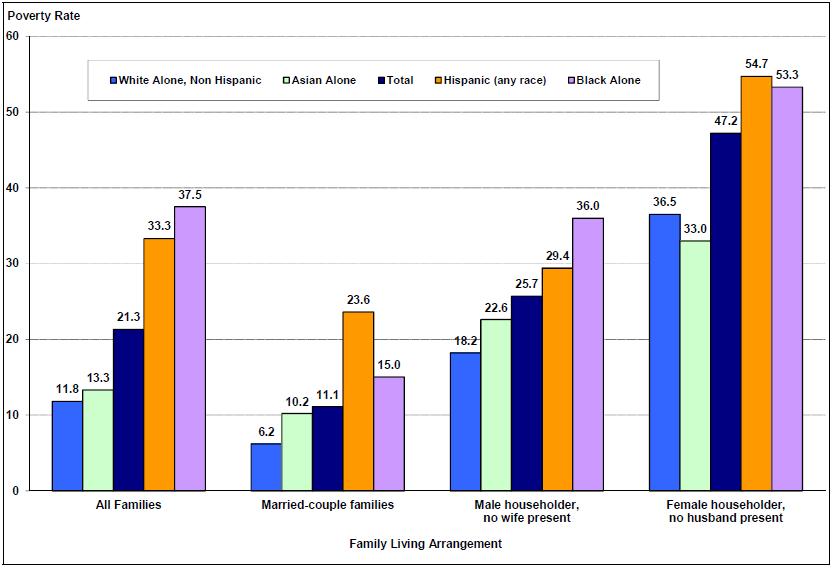
Children living in single female-headed families are especially prone to poverty. In 2012 a child living in a single female-headed family was well over four times more likely to be poor than a child living in a married-couple family. In 2012, among all children living in single female-headed families, 47.2% were poor. In contrast, among children living in married-couple families, 11.1% were poor. The increased share of children who live in single female-headed families has contributed to the high overall child poverty rate. In 2012, one quarter (25.3%) of children were living in single female-headed families, more than double the share who lived in such families when the overall child poverty rate was at a historical low (1969). Among all poor children, well over half (56.1%) were living in single female-headed families in 2012.
In 2012, 37.5% of black children were poor (4.1 million), compared to 33.3% of Hispanic children (5.7 million) and 11.8% of non-Hispanic white children (4.4 million). (See Figure 3.) Among children living in single female-headed families, more than half of black children (53.3%) and Hispanic children (54.7%) were poor; in contrast, over one-third of non-Hispanic white children (36.5%) were poor. The poverty rate among Hispanic children who live in married-couple families (23.6%) was about half-again as high as that of black children (15.0%), and nearly four times that of non-Hispanic white children (6.2%) who live in such families. Contributing to the high rate of overall black child poverty is the large share of black children who live in single female-headed families (54.3%) compared to Hispanic children (29.6%) or non-Hispanic white children (16.1%). (See Figure 4.)
Figure 3. Child Poverty Rates by Family Living Arrangement, Race and Hispanic Origin, 2012
Source: Figure prepared by the Congressional Research Service (CRS) based on U.S. Census Bureau data from the 2013 Current Population Survey Annual Social and Economic Supplement, available at http://www.census.gov/hhes/www/cpstables/032013/pov/pov05_000.htm.
Figure 4. Composition of Children, by Family Type, Race and Hispanic Origin, 2012
Source: Figure prepared by the Congressional Research Service (CRS) based on U.S. Census Bureau data from the 20l3 Current Population Survey Annual Social and Economic Supplement, available at http://www.census.gov/hhes/www/cpstables/032013/pov/pov05_100.htm.
Adults with Low Education, Unemployment, or Disability
Adults with low education, those who are unemployed, or those who have a work-related disability are especially prone to poverty. In 2012 among 25- to 34-year-olds without a high school diploma, about 2 out of 5 (39.1%) were poor. Within the same age group, over 1 of 5 (21.5%) whose highest level of educational attainment was a high school diploma were poor. In contrast, only about 1 in 18 (5.6%) of 25- to 34-year-olds with at least a bachelor's degree were found to be living below the poverty line. (About 11% of 25- to 34-year-olds lack a high school diploma.) Among persons between the ages of 16 and 64 who were unemployed in March 2013, nearly 3 out of 10 (28.6%) were poor based on their families' incomes in 2012; among those who were employed, 7.0% were poor. In 2012, persons who had a work disability |11| represented 11.3% of the 16- to 64-year-old population, and about one-quarter (25.3%) of the poor population within this age range. Among those with a severe work disability, 34.9% were poor, compared to 16.7% of those with a less severe disability and 11.6% who reported having no work-related disability.
In spite of the recession, the poverty rate among the aged remained at a historic low of 9.1% in 2012 (statistically tied with the 2011 rate of 8.7%). In 2012, an estimated 3.9 million persons age 65 and older were considered poor under the "official" poverty measure. Among persons age 75 and over, 10.6% were poor in 2012, compared to 7.9% of those ages 65 to 74. Many of the aged live just slightly above the poverty line. As measured by a slightly raised poverty standard (125% of the poverty threshold), 14.8% of the aged could be considered poor or "near poor"; 12.1% who are ages 65 to 74, and 17.8% who are 75 years of age and over, could be considered poor or "near poor."
Receipt of Need-Tested Assistance Among the Poor
In 2012, among poor persons, nearly three of every four (74.4%) lived in households that received any means-tested assistance during the year. |12| Such assistance could include cash aid, such as Temporary Assistance for Needy Families (TANF), Supplemental Security Income (SSI) payments, SNAP benefits (Food Stamps), Medicaid, subsidized housing, free or reduced price school lunches, and other programs. In 2012, fewer than 1 in 5 (18.5%) poor persons lived in households that received cash aid; half (50.6%) received SNAP benefits (formerly named Food Stamps); 6 in 10 (61.8%) lived in households where one or more household members were covered by Medicaid; and about 1 in 7 (14.9%) lived in subsidized housing. Poor single-parent families with children are among those families most likely to receive cash aid. Among poor children who were living in single female-headed families, one-quarter (24.0%) were in households that received government cash aid in 2012. The share of poor children in single female-headed families receiving cash aid is well below historical levels. In 1993, 70.2% of these children's families received cash aid. In 1995, the year prior to passage of sweeping welfare changes under PRWORA, 65% of such children were in families receiving cash aid.
Poverty is more highly concentrated in some areas than in others; it is about twice as high in center cities as it is in suburban areas and nearly three times as high in the poorest states as it is in the least poor states. Some neighborhoods may be characterized as having high concentrations of poverty. Among the poor, the likelihood of living in an area of concentrated or extreme poverty varies by race and ethnicity.
Poverty in Metropolitan and Nonmetropolitan Areas, Center Cities, and Suburbs
Within metropolitan areas, the incidence of poverty in central city areas is considerably higher than in suburban areas--19.7% versus 11.2%, respectively, in 2012. Nonmetropolitan areas had a poverty rate of 17.7%. A typical pattern is for poverty rates to be highest in center city areas, with poverty rates dropping off in suburban areas, and then rising with increasing distance from an urban core.
In 2012, poverty rates were lowest in the Northeast (13.6%), followed by the Midwest (13.3%), and the West (15.1%), with the South having the highest poverty rate (16.5%). Among the four regions, only the West experienced statistically significant change in its poverty rate from 2011 to 2012, with its rate declining from 15.8% to 15.1% over the period.
American Community Survey (ACS) State Poverty Estimates--2012 Up to this point, the poverty statistics presented in this report come from the U.S. Census Bureau's Annual Social and Economic Supplement (ASEC) to the Current Population Survey (CPS). For purposes of producing state and sub-state poverty estimates, the Census Bureau now recommends using the American Community Survey (ACS)-- because of its much larger sample size, the ACS produces estimates with a much smaller margin of statistical error than that of the CPS/ASEC. However, it should be noted that the ACS survey design differs from the CPS/ASEC in a variety of ways, and may produce somewhat different estimates than those obtained from the ASEC/CPS. Based on the 2012 ACS, the U.S. poverty rate was estimated to be 15.9%, compared to 15.0% based on the 2013 CPS/ASEC. The CPS/ASEC estimates are based on a survey conducted in February through April 2013, and account for income reported for the previous year. In contrast, the ACS estimates are based on income information collected between January and December 2012, for the prior 12 months. For example, for the sample with data collected in January, the reference period is from January 2011 to December 2011, and for the sample with data collected in December, from December 2011 to November 2012. The ACS data consequently cover a time span of 23 months, with the data centered at mid-December 2011.
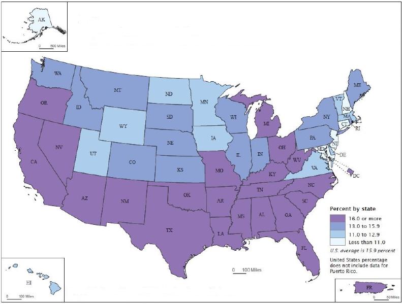
Based on 2012 American Community Survey (ACS) data, poverty rates were highest in the South (with the exception of Virginia), extending across to Southwestern states bordering Mexico (Texas, New Mexico, and Arizona). (See Figure 5.) Poverty rates in several states bordering the Ohio River (Ohio, West Virginia, Kentucky) also exceeded the national rate, as did those of Michigan and the District of Columbia, in the eastern half of the nation, and California, Oregon, and Nevada in the western half.
States along the Atlantic Seaboard from Virginia northward tended to have poverty rates well below the national rate, as did three contiguous states in the upper Midwest/plains (Iowa, Minnesota, and North Dakota), as well as Utah, Wyoming, Alaska, and Hawaii.
Figure 5. Percentage of People in Poverty in the Past 12 Months by State and Puerto Rico: 2012
Source: U.S. Census Bureau, 2011 American Community Survey, 2012 Puerto Rico Community Survey. Alemayehu Bishaw, Poverty: 2000 to 2012, U.S. Census Bureau, American Community Survey Briefs, ACSBR/12 01, Washington, DC, September 2013, p. 5, http://www.census.gov/prod/20l3pubs/acsbrl2-0l.pdf
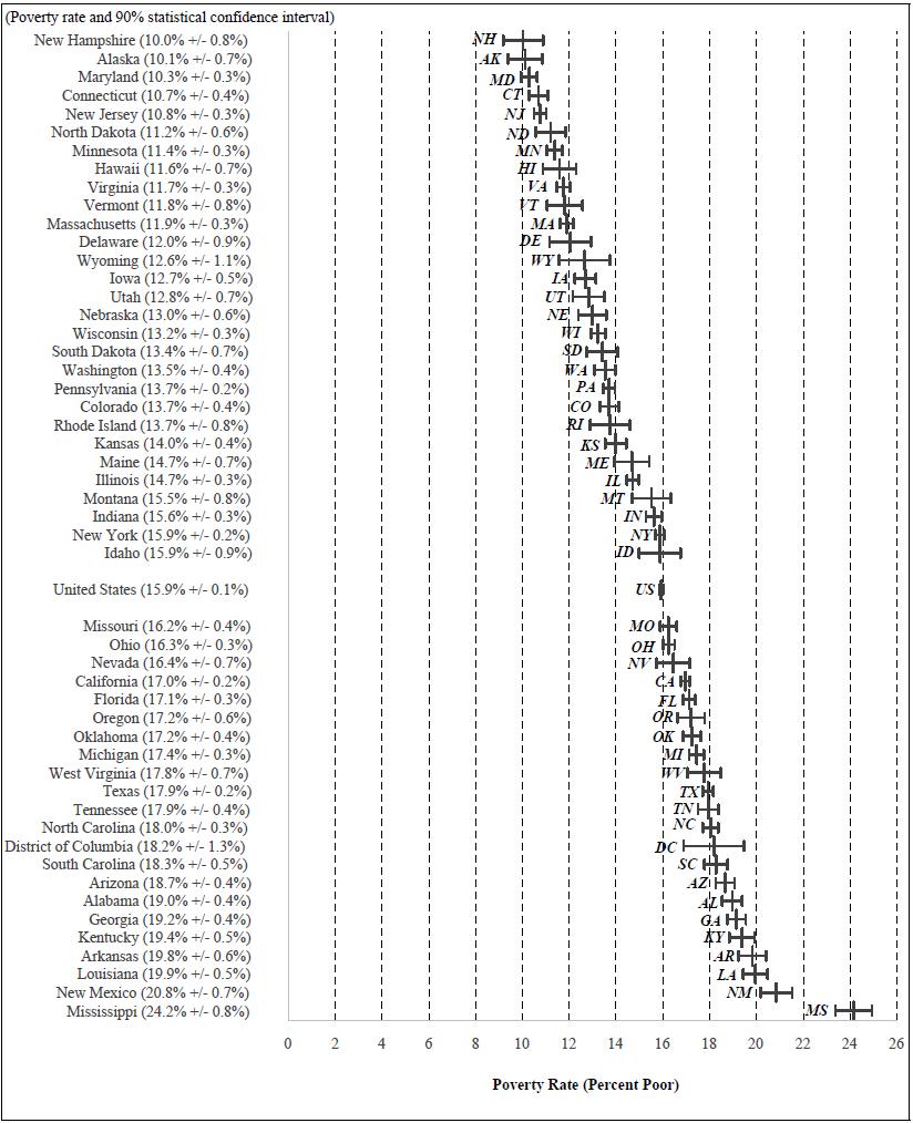
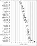
Figure 6 shows estimated poverty rates for the United States and for each of the 50 states and the District of Columbia on the basis of the 2012 American Community Survey (ACS), the most recent ACS data currently available. In addition to the point estimates, the figure displays a 90% statistical confidence interval around each state's estimate, indicating the degree to which these estimates might be expected to vary based on sample size. Although the states are sorted from lowest to highest by their respective poverty rate point estimates, the precise ranking of each state is not possible because of the depicted margin of error around each state's estimate. All states with non-overlapping statistical confidence intervals have statistically significant different poverty rates from one another. Some states with overlapping confidence intervals may also have significantly different poverty rates from one another, measured at the 90% confidence interval. |13|
For example, New Hampshire, shown as having the lowest poverty rate (10.0%) in 2012, is statistically tied with several other states, including Alaska (10.1%), Maryland (10.3%), Connecticut (10.6%), and New Jersey (10.8%). Mississippi clearly stands out as the state with the highest poverty rate (24.2%). New Mexico, with a poverty rate of 20.8%, has the second-highest poverty rate, and is statistically untied with any other state, even though its statistical confidence interval overlaps with several other states. Louisiana, a state ranked as having the third-highest poverty rate (19.9%), is statistically tied with Arkansas (19.8%) and Kentucky (19.4%), but not with Georgia (19.2) nor Alabama (19.0), even though their statistical confidence intervals overlap.
Figure 6. Poverty Rates for the 50 States and the District of Columbia: 2012 American Community Survey (ACS) Data
Source: Prepared by the Congressional Research Service on the basis of U.S. Census Bureau 20l2 American Community Survey (ACS) data.
Change in State Poverty Rates: 2002-2012
Table 1 provides estimates of state and national poverty rates from 2002 through 2012 from the ACS. Statistically significant changes from one year to the next are indicated by an upward-pointing arrow (▲) if a state's poverty rate was statistically higher, and by a downward-pointing arrow (▼) if statistically lower, than in the immediately preceding year or for other selected periods (i.e., 2005 vs. 2002, 2011 vs. 2007). |14| It should be noted that ACS poverty estimates for 2006 and later are not strictly comparable to those of earlier years, due to a change in ACS methodology that began in 2006 to include some persons living in non-institutionalized group quarters who were not included in earlier years. |15|
Table 1 shows that three states (California, Mississippi, and New Hampshire) experienced statistically significant increases in their poverty rates from the 2011 to 2012 ACS. California's estimated poverty rate increased form 16.6% in 2011, to 17.0% in 2012, while Mississippi's rate increased from 22.6% to 24.2%, and New Hampshire's rate increased from 8.8% to 10.0%, over the period. Two states (Minnesota and Texas) experienced statistically significant decreases in their poverty rates from 2011 to 2012, with Minnesota's rate falling from 11.9% to 11.4%, and Texas's rate falling from 18.5% to 17.9% over the period.
The table shows that poverty among states generally increased over the 2002 to 2005 period, as measured by the ACS, consequent to the 2001 (March to November) economic recession. From the 2002 to 2003 ACS, five states (including the District of Columbia) experienced statistically significant increases in their poverty rates, whereas none experienced a statistically significant decrease. From 2003 to 2004, eight states saw their poverty rates increase, whereas two saw decreases. From 2004 to 2005, 13 states saw their poverty rates increase, whereas only 1 saw its poverty rate decrease. Comparing poverty rates from the 2005 ACS to those from the 2002 ACS, poverty was statistically higher in 25 states, and lower in only 2.
By 2007, poverty rates among states were beginning to improve, with 13 states (including the District of Columbia) experiencing statistically significant declines in their poverty rates from 2006; only Michigan experienced a statistically significant increase in its poverty rate in 2007 compared to a year earlier.
Since 2007, state poverty rates have generally increased consequent to the 18-month recession (December 2007 to June 2009). From 2007 to 2008, the ACS data showed eight states (California, Connecticut, Florida, Hawaii, Indiana, Michigan, Oregon, and Pennsylvania) as experiencing statistically significant increases in their poverty rates, whereas three states (Alabama, Louisiana, and Texas) experienced statistically significant decreases. From 2008 to 2009, 32 states saw their poverty rates increase, and no state experienced a statistically significant decrease, and from 2009 to 2010, 34 states experienced statistically significant increases in poverty, and again, no state experienced a decrease. As noted above, from 2011 to 2012, three states saw their poverty rates rise, and only two saw a decline. Comparing 2012 to 2007, poverty rates were statistically higher in 47 states (including the District of Columbia), and no state had a poverty rate statistically below its prerecession rate.
Table 1. Poverty Rates for the 50 States and the District of Columbia, 2002 to 2012 Estimates from the American Community Survey (ACS)
(percent poor)
Estimated Poverty Rates and Statistically Significant Differences over Previous Year Change in Poverty Rates
over Selected Periods
and Statistically
Significant Differencesa2002 2003 2004 2005 2006b 2007b 2008b 2009b 2010b 2011b 2012b 2005
vs.
20112012
vs.
2007
United States
12.4
12.7 ▲
13.1 ▲
13.3 ▲
13.3
13.0 ▼
13.2 ▲
14.3 ▲
15.3 ▲
15.9 ▲
15.9
0.9 ▲
3.0 ▲Alabama 16.6 17.1 16.1 17.0 ▲ 16.6 16.9 15.7 ▼ 17.5 ▲ 19.0 ▲ 19.0 19.0 -0.1 2.1 ▲ Alaska 7.7 9.7 ▲ 8.2 ▼ 11.2 ▲ 10.9 8.9 ▼ 8.4 9.0 9.9 10.5 10.1 3.2 ▲ 1.2 ▲ Arizona 14.2 15.4 ▲ 14.2 14.2 14.2 14.2 14.7 16.5 ▲ 17.4 ▲ 19.0 ▲ 18.7 0.0 4.5 ▲ Arkansas 15.3 16.0 17.9 ▲ 17.2 17.3 17.9 17.3 18.8 ▲ 18.8 19.5 19.8 2.0 ▲ 2.0 ▲ California 13.0 13.4 13.3 13.3 13.1 12.4 ▼ 13.3 ▲ 14.2 ▲ 15.8 ▲ 16.6 ▲ 17.0 ▲ 0.1 4.6 ▲ Colorado 9.7 9.8 11.1 11.1 12.0 ▲ 12.0 11.4 12.9 ▲ 13.4 13.5 13.7 2.3 ▲ 1.7 ▲ Connecticut 7.5 8.1 7.6 8.3 8.3 7.9 9.3 ▲ 9.4 10.1 ▲ 10.9 ▲ 10.7 0.8 2.8 ▲ Delaware 8.2 8.7 9.9 10.4 11.1 10.5 10.0 10.8 11.8 11.9 12.0 2.9 ▲ 1.6 ▲ Dist. of Col. 17.5 19.9 ▲ 18.9 19.0 19.6 16.4 ▼ 17.2 18.4 19.2 18.7 18.2 2.2 1.7 Florida 12.8 13.1 12.2 ▼ 12.8 ▲ 12.6 12.1 ▼ 13.2 ▲ 14.9 ▲ 16.5 ▲ 17.0 ▲ 17.1 -0.2 5.0 ▲ Georgia 12.7 13.4 14.8 ▲ 14.4 14.7 14.3 14.7 16.5 ▲ 17.9 ▲ 19.1 ▲ 19.2 2.0 ▲ 4.9 ▲ Hawaii 10.1 10.9 10.6 9.8 9.3 8.0 ▼ 9.1 ▲ 10.4 ▲ 10.7 12.0 11.6 -0.8 3.6 ▲ Idaho 13.8 13.8 14.5 13.9 12.6 ▼ 12.1 12.6 14.3 ▲ 15.7 ▲ 16.5 15.9 -1.2 3.7 ▲ Illinois 11.6 11.3 11.9 12.0 12.3 11.9 12.2 13.3 ▲ 13.8 ▲ 15.0 ▲ 14.7 0.7 ▲ 2.8 ▲ Indiana 10.9 10.6 10.8 12.2 ▲ 12.7 12.3 13.1 ▲ 14.4 ▲ 15.3 ▲ 16.0 ▲ 15.6 1.8 ▲ 3.3 ▲ Iowa 11.2 10.1 9.9 10.9 ▲ 11.0 11.0 11.5 11.8 12.6 ▲ 12.8 12.7 -0.2 1.7 ▲ Kansas 12.1 10.8 10.5 11.7 ▲ 12.4 11.2 ▼ 11.3 13.4 ▲ 13.6 13.8 14.0 0.3 2.8 ▲ Kentucky 15.6 17.4 17.4 16.8 17.0 17.3 17.3 18.6 ▲ 19.0 19.1 19.4 1.3 ▲ 2.1 ▲ Louisiana 18.8 20.3 19.4 19.8 19.0 18.6 17.3 ▼ 17.3 18.7 ▲ 20.4 ▲ 19.9 0.2 1.3 ▲ Maine 11.1 10.5 12.3 ▲ 12.6 12.9 12.0 12.3 12.3 12.9 14.1 ▲ 14.7 1.8 ▲ 2.6 ▲ Maryland 8.1 8.2 8.8 8.2 7.8 8.3 8.1 9.1 ▲ 9.9 ▲ 10.1 10.3 -0.3 2.0 ▲ Massachusetts 8.9 9.4 9.2 10.3 ▲ 9.9 9.9 10.0 10.3 11.4 ▲ 11.6 11.9 1.0 ▲ 1.9 ▲ Michigan 11.0 11.4 12.3 13.2 ▲ 13.5 14.0 ▲ 14.4 ▲ 16.2 ▲ 16.8 ▲ 17.5 ▲ 17.4 2.5 ▲ 3.4 ▲ Minnesota 8.5 7.8 8.3 9.2 ▲ 9.8 ▲ 9.5 9.6 11.0 ▲ 11.6 ▲ 11.9 11.4 ▼ 1.2 ▲ 1.9 ▲ Mississippi 19.9 19.9 21.6 ▲ 21.3 21.1 20.6 21.2 21.9 22.4 22.6 24.2 ▲ 1.2 ▲ 3.5 ▲ Missouri 11.9 11.7 11.8 13.3 ▲ 13.6 13.0 ▼ 13.4 14.6 ▲ 15.3 ▲ 15.8 16.2 1.6 ▲ 3.2 ▲ Montana 14.6 14.2 14.2 14.4 13.6 14.1 14.8 15.1 14.6 14.8 15.5 -1.0 1.4 ▲ Nebraska 11.0 10.8 11.0 10.9 11.5 11.2 10.8 12.3 ▲ 12.9 13.1 13.0 0.5 1.8 ▲ Nevada 11.8 11.5 12.6 11.1 10.3 10.7 11.3 12.4 ▲ 14.9 ▲ 15.9 16.4 -1.5 ▼ 5.8 ▲ New Hampshire 6.4 7.7 ▲ 7.6 7.5 8.0 7.1 ▼ 7.6 8.5 ▲ 8.3 8.8 10.0 ▲ 1.6 ▲ 3.0 ▲ New Jersey 7.5 8.4 ▲ 8.5 8.7 8.7 8.6 8.7 9.4 ▲ 10.3 ▲ 10.4 10.8 1.2 ▲ 2.2 ▲ New Mexico 18.9 18.6 19.3 18.5 18.5 18.1 17.1 18.0 20.4 ▲ 21.5 20.8 -0.4 2.7 ▲ New York 13.1 13.5 14.2 ▲ 13.8 14.2 ▲ 13.7 ▼ 13.6 14.2 ▲ 14.9 ▲ 16.0 ▲ 15.9 1.1 ▲ 2.2 ▲ North Carolina 14.2 14.0 15.2 15.1 14.7 14.3 14.6 16.3 ▲ 17.5 ▲ 17.9 18.0 0.4 3.7 ▲ North Dakota 12.5 11.7 12.1 11.2 11.4 12.1 12.0 11.7 13.0 ▲ 12.2 11.2 -1.1 -0.9 Ohio 11.9 12.1 12.5 13.0 13.3 13.1 13.4 15.2 ▲ 15.8 ▲ 16.4 ▲ 16.3 1.5 ▲ 3.1 ▲ Oklahoma 15.0 16.1 15.3 16.5 17.0 15.9 ▼ 15.9 16.2 16.9 ▲ 17.2 17.2 2.0 ▲ 1.3 ▲ Oregon 13.2 13.9 14.1 14.1 13.3 ▼ 12.9 13.6 ▲ 14.3 15.8 ▲ 17.5 ▲ 17.2 0.0 4.3 ▲ Pennsylvania 10.5 10.9 11.7 ▲ 11.9 12.1 11.6 ▼ 12.1 ▲ 12.5 ▲ 13.4 ▲ 13.8 13.7 1.5 ▲ 2.1 ▲ Rhode Island 10.7 11.3 12.8 ▲ 12.3 11.1 12.0 11.7 11.5 14.0 ▲ 14.7 13.7 0.4 1.8 ▲ South Carolina 14.2 14.1 15.7 15.6 15.7 15.0 15.7 17.1 ▲ 18.2 ▲ 18.9 ▲ 18.3 1.4 ▲ 3.2 ▲ South Dakota 11.4 11.1 11.0 13.6 ▲ 13.6 13.1 12.5 14.2 ▲ 14.4 13.9 13.4 2.2 0.3 Tennessee 14.5 13.8 14.5 15.5 16.2 15.9 15.5 17.1 ▲ 17.7 18.3 17.9 1.7 ▲ 2.0 ▲ Texas 15.6 16.3 16.6 17.6 ▲ 16.9 ▼ 16.3 ▼ 15.8 ▼ 17.2 ▲ 17.9 ▲ 18.5 ▲ 17.9 ▼ 1.3 ▲ 1.6 ▲ Utah 10.5 10.6 10.9 10.2 10.6 9.7 ▼ 9.6 11.5 ▲ 13.2 ▲ 13.5 12.8 0.1 3.2 ▲ Vermont 8.5 9.7 9.0 11.5 ▲ 10.3 10.1 10.6 11.4 12.7 ▲ 11.5 ▼ 11.8 1.8 ▲ 1.7 ▲ Virginia 9.9 9.0 9.5 10.0 9.6 9.9 10.2 10.5 11.1 ▲ 11.5 ▲ 11.7 -0.4 1.8 ▲ Washington 11.4 11.0 13.1 ▲ 11.9 ▼ 11.8 11.4 11.3 12.3 ▲ 13.4 ▲ 13.9 13.5 0.4 2.1 ▲ West Virginia 17.2 18.5 17.9 18.0 17.3 16.9 17.0 17.7 18.1 18.6 17.8 0.1 0.9 Wisconsin 9.7 10.5 10.7 10.2 11.0 ▲ 10.8 10.4 12.4 ▲ 13.2 ▲ 13.1 13.2 1.2 ▲ 2.4 ▲ Wyoming 11.0 9.7 10.3 9.5 9.4 8.7 9.4 9.8 11.2 11.3 12.6 -1.6 ▼ 4.0 ▲ Number of states
with statistically
significant change
in poverty5 10 14 7 14 11 32 34 18 5 27 47
Increase in poverty
5 ▲
8 ▲
13 ▲
4 ▲
1 ▲
8 ▲
32 ▲
34 ▲
17 ▲
3 ▲
25 ▲
47 ▲Decrease in poverty 0 ▼ 2 ▼ 1 ▼ 3 ▼ 13 ▼ 3 ▼ 0 ▼ 0 ▼ 1 ▼ 2 ▼ 2 ▼ 0 ▼ Source: Congressional Research Service (CRS) estimates from U.S. Census Bureau American Community Survey (ACS) data, 2002 to 20I2.
Notes: ▲ Statistically significant increase in poverty rate at the 90% statistical confidence level.
▼ Statistically significant decrease in poverty rate at the 90% statistical confidence level.
a. Depicted changes in poverty rates over selected periods may differ slightly from differences calculated directly from the table, due to rounding.
b. Comparisons to 2002 through 2005 estimates are not strictly comparable, due to inclusion of persons living in some non-institutional group quarters beginning in 2006 and after.Poverty Rates by Metropolitan Area
The four tables that follow provide poverty estimates for large metropolitan areas having a population of 500,000 and over, and for smaller metropolitan areas having a population of 50,000 or more but less than 500,000. Among large metropolitan areas, 10 areas with some of the lowest poverty rates are shown in Table 2, and the 10 areas with some of the highest poverty rates are shown in Table 3. Among smaller metropolitan areas, 10 areas with some of the lowest poverty rates are shown in Table 4, and 10 among those with the highest poverty rates in Table 5. It should be noted that metropolitan areas shown in these tables may not be statistically different from one another, or from others not shown in the tables.
Poverty estimates for all metropolitan areas are shown in Appendix B. Table B-1 includes poverty rate estimates for 2012, and whether 2012 estimates statistically differ from 2011. The table shows that from 2011 to 2012, 26 metropolitan areas experienced statistically significant increases in their poverty rates, whereas 25 areas experienced statistically significant decreases.
Table 2. Large Metropolitan Areas Among Those with the Lowest Poverty Rates: 2012
(Metropolitan Areas with Population of 500,000 and Over)
Metropolitan Area Total Population Number Poor Poverty Rate (Percent Poor) Estimate Margin of Errora Estimate Margin of Errora Washington-Arlington-Alexandria, DC-VA-MD-WV 5,702,639 477,661 +/-17,577 8.4% +/-0.3% Bridgeport-Stamford-Norwalk, CT 915,813 81,629 +/-7,143 8.9% +/-0.8% Ogden-Clearfield, UT 556,266 56,638 +/-7,028 10.2% +/-1.3% Honolulu, HI 945,975 97,754 +/-8,616 10.3% +/-0.9% Allentown-Bethlehem-Easton, PA-NJ 804,602 84,127 +/-6,553 10.5% +/-0.8% Boston-Cambridge-Quincy, MA-NH 4,486,468 479,126 +/-15,238 10.7% +/-0.3% Minneapolis-St. Paul-Bloomington, MN-WI 3,299,784 352,560 +/-14,086 10.7% +/-0.4% San Jose-Sunnyvale-Santa Clara, CA 1,868,187 202,357 +/-12,662 10.8% +/-0.7% Hartford-West Hartford-East Hartford, CT 1,169,356 127,371 +/-7,291 10.9% +/-0.6% Albany-Schenectady-Troy, NY 843,802 93,228 +/-6,350 11.0% +/-0.8% Source: Table prepared by the Congressional Research Service (CRS) based on analysis of U.S. Census Bureau 2012 American Community Survey (ACS) data, table series S1701: Poverty Status in the Past 12 Months, from the Census Bureau's American FactFinder, available at http://factfinder2.census.gov/faces/nav/jsf/pages/index.xhtml.
Notes: Areas are included based on their estimated 2012 poverty rates. Areas shown may not be statistically different from one another, or from others not shown in the table.
a. Margin of error of an estimate based on a 90% statistical confidence level. When added to and subtracted from an estimate, the range reflects a 90% statistical confidence interval bounding the estimate.
Table 3. Large Metropolitan Areas Among Those with the Highest Poverty Rates: 2012
(Metropolitan Areas with Population of 500,000 and Over)
Metropolitan Area Total Population Number Poor Poverty Rate (Percent Poor) Estimate Margin of Errora Estimate Margin of Errora McAllen-Edinburg-Mission, TX 796,479 274,713 +/-17,146 34.5% +/-2.2% Fresno, CA 930,872 264,738 +/-13,321 28.4% +/-1.4% El Paso, TX 812,645 195,247 +/-10,809 24.0% +/-1.3% Bakersfield-Delano, CA 825,020 196,625 +/-13,837 23.8% +/-2.2% Jackson, MS 531,354 117,984 +/-8,520 22.2% +/-1.6% Modesto, CA 515,955 104,559 +/-10,039 20.3% +/-1.9% Augusta-Richmond County, GA-SC 553,981 112,218 +/-8,963 20.3% +/-1.6% Tucson, AZ 968,447 193,466 +/-11,146 20.0% +/-1.1% Toledo, OH 630,598 125,508 +/-7,513 19.9% +/-1.2% Memphis, TN-MS-AR 1,307,830 259,780 +/-10,892 19.9% +/-0.8% Source: Table prepared by the Congressional Research Service (CRS) based on analysis of U.S. Census Bureau 2012 American Community Survey (ACS) data, table series S1701: Poverty Status in the Past 12 Months, from the Census Bureau's American FactFinder, available at http://factfinder2.census.gov/faces/nav/jsf/pages/index.xhtml.
Notes: Areas are included based on their estimated 20I2 poverty rates. Areas shown may not be statistically different from one another, or from others not shown in the table.
a. Margin of error of an estimate based on a 90% statistical confidence level. When added to and subtracted from an estimate, the range reflects a 90% statistical confidence interval bounding the estimate.
Table 4. Smaller Metropolitan Areas Among Those with the Lowest Poverty Rates: 2012
(Metropolitan Areas with Populations Between 50,000 and 499,999)
Metropolitan Area Total Population Number Poor Poverty Rate (Percent Poor) Estimate Margin of Errora Estimate Margin of Errora Midland, TX 145,188 9,086 +/-2,649 6.3% +/-1.8% Bismarck, ND 110,290 7,266 +/-1,572 6.6% +/-1.4% Fairbanks, AK 96,529 6,646 +/-1,813 6.9% +/-1.9% Appleton, WI 225,045 18,885 +/-2,630 8.4% +/-1.2% Anchorage, AK 384,749 33,353 +/-4,104 8.7% +/-1.1% Fond du Lac, WI 98,703 8,608 +/-1,938 8.7% +/-2.0% Napa, CA 135,439 11,996 +/-2,747 8.9% +/-2.0% Ocean City, NJ 93,825 8,392 +/-2,201 8.9% +/-2.3% Norwich-New London, CT 262,896 24,105 +/-3,537 9.2% +/-1.3% Cedar Rapids, IA 254,225 24,150 +/-3,246 9.5% +/-1.3% Source: Table prepared by the Congressional Research Service (CRS) based on analysis of U.S. Census Bureau 2012 American Community Survey (ACS) data, table series S1701: Poverty Status in the Past 12 Months, from the Census Bureau's American FactFinder, available at http://factfinder2.census.gov/faces/nav/jsf/pages/index.xhtml.
Notes: Areas are included based on their estimated 2012 poverty rates. Areas shown may not be statistically different from one another, or from others not shown in the table.
a. Margin of error of an estimate based on a 90% statistical confidence level. When added to and subtracted from an estimate, the range reflects a 90% statistical confidence interval bounding the estimate.
Table 5. Smaller Metropolitan Areas Among Those with the Highest Poverty Rates: 2012
(Metropolitan Areas with Population of 500,000 and Over)
Metropolitan Area Total Population Number Poor Poverty Rate (Percent Poor) Estimate Margin of Errora Estimate Margin of Errora Brownsville-Harlingen, TX 411,003 148,267 +/-9,666 36.1% +/-2.3% Laredo, TX 254,758 81,651 +/-7,394 32.1% +/-2.9% Visalia-Porterville, CA 444,186 135,194 +/-9,353 30.4% +/-2.1% Gainesville, FL 254,375 70,552 +/-5,754 27.7% +/-2.2% Las Cruces, NM 209,622 56,903 +/-6,722 27.1% +/-3.2% Albany, GA 148,869 40,011 +/-4, 170 26.9% +/-2.8% College Station-Bryan, TX 219,226 57,006 +/-5, 130 26.0% +/-2.3% Flagstaff, AZ 127,795 33,191 +/-4,344 26.0% +/-3.4% Monroe, LA 168,014 43,435 +/-5,407 25.9% +/-3.2% Hattiesburg, MS 143,389 36,577 +/-4,869 25.5% +/-3.4% Source: Table prepared by the Congressional Research Service (CRS) based on analysis of U.S. Census Bureau 2012 American Community Survey (ACS) data, table series S1701: Poverty Status in the Past 12 Months, from the Census Bureau's American FactFinder, available at http://factfinder2.census.gov/faces/nav/jsf/pages/index.xhtml.
Notes: Areas are included based on their estimated 20I2 poverty rates. Areas shown may not be statistically different from one another, or from others not shown in the table.
a. Margin of error of an estimate based on a 90% statistical confidence level. When added to and subtracted from an estimate, the range reflects a 90% statistical confidence interval bounding the estimate.
Congressional District Poverty Estimates
Poverty estimates for congressional districts are shown in Appendix C. Table C-1 includes poverty rate estimates for 2012. Congressional districts in 2012 are not directly comparable to earlier years, due to re-districting.
"Neighborhood" Poverty--Poverty Areas and Areas of Concentrated and Extreme Poverty
The estimates presented here are based on five years of American Community Survey (ACS) data (2006-2010 ACS), and will be updated once the Census Bureau releases 5-year ACS estimates for 2008-2012, in December 2013. Neighborhoods can be delineated from U.S. Census Bureau census tracts. Census tracts usually have between 2,500 and 8,000 persons and, when first delineated, are designed to be homogeneous with respect to population characteristics, economic status, and living conditions. The Census Bureau defines "poverty areas" as census tracts having poverty rates of 20% or more.
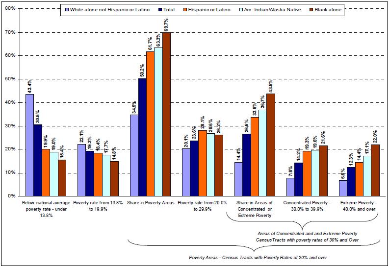
Figure 7 groups census tracts according to their level of poverty. The first two groupings are based on poor persons living in census tracts with poverty rates below the national average (13.8% based on the five-year ACS data), and from 13.8% to less than 20.0%. Poor persons living in census tracts with poverty rates of 20% or more meet the Census Bureau definition of living in "poverty areas." Poverty areas are further demarcated in terms of poor persons living in areas of "concentrated" poverty (i.e., census tracts with poverty rates of 30% to 39.9%), and areas of "extreme" poverty (i.e., census tracts with poverty rates of 40% or more). The figure is based on five years of data (2006-2010) from the U.S. Census Bureau's American Community Survey (ACS). Five years of data are required in order to get reasonably reliable statistical data at the census tract level while at the same time preserving the confidentiality of survey respondents.
Figure 7. Distribution of Poor People by Race and Hispanic Origin, by Level of Neighborhood (Census Tract) Poverty, 2006-2010
Source: Congressional Research Service (CRS) analysis of U.S. Census Bureau American Community Survey, five-year (2006-2010) data.
Figure 7 shows that over the five-year period 2006-2010, half of all poor persons (50.2%) lived in "poverty areas" (i.e., census tracts with poverty rates of 20% or more). Over one-quarter (26.5%) lived in areas with poverty of 30% or more, and about one in eight (12.3%) lived in areas of "extreme" poverty, having poverty rates of 40% or more. Among the poor, African Americans, American Indian and Alaska Natives, and Hispanics are more likely to live in poverty areas than either Asians or white non-Hispanics. Among poor blacks, over two of every five (43.5%) live in neighborhoods with poverty rates of 30% or more, and over one in five (22.0%) live in "extreme" poverty areas, with poverty rates of 40% or more. Among Hispanics, one-third (33.6%) live in areas with poverty rates of 30% or more, and about one in seven (14.4%) live in areas of "extreme" poverty. Among white non-Hispanics, close to two-thirds (64.5%) live outside poverty areas, while about one in seven (14.4%) live in areas with poverty rates of 30% or more.
The Research Supplemental Poverty Measure
On November 6, 2013, the Census Bureau released its third annual report using a new Supplemental Poverty Measure (SPM). |16| As its name implies, the SPM is intended to "supplement," rather than replace, the "official" poverty measure. The "official" Census Bureau statistical measure of poverty will continue to be used by programs that allocate funds to states or other jurisdictions on the basis of poverty, and the Department of Health and Human Services (HHS) will continue to derive Poverty Income Guidelines from the "official" Census Bureau measure.
Many experts consider the "official" poverty measure to be flawed and outmoded. |17| In 1990, Congress commissioned a study on how poverty is measured in the United States, resulting in the National Academy of Sciences (NAS) convening a 12-member expert panel to study the issue. The NAS panel issued a wide range of specific recommendations to develop an improved statistical measure of poverty in its 1995 report Measuring Poverty: A New Approach. |18|
In late 2009, the Office of Management and Budget (OMB) formed an Interagency Technical Working Group |19| (ITWG) to suggest how the Census Bureau, in cooperation with the Bureau of Labor Statistics (BLS), should develop a new Supplemental Poverty Measure, using the NAS expert panel's recommendations as a starting point. Referencing the work of the ITWG, |20| the Department of Commerce announced in March 2010 that the Census Bureau was developing a new Supplemental Poverty Measure, as "an alternative lens to understand poverty and measure the effects of anti-poverty policies," with the intention that the new measure "will be dynamic and will benefit from improvements over time based on new data and new methodologies." |21|
The SPM is intended to address a number of weaknesses of the "official" measure. Criticisms of the "official" poverty measure raised by the NAS expert panel include the following:
- The "official" poverty measure, by counting only families' total cash, pre-tax income as a resource in determining poverty status, ignores a host of government programs and policies that affect the disposable income families may actually have available. For example, the official measure ignores the effects of payroll taxes paid by families, and tax benefits they may receive such as the EITC and the Child Tax Credit. It ignores a variety of in-kind benefits, such as SNAP benefits and free or reduced-price lunches under the National School Lunch Program, that free up resources to meet other needs. Similarly, it ignores housing subsidies that help make housing more affordable.
- The "official" poverty income thresholds used in determining families' and individuals' poverty status, devised in the early 1960s, have changed little since. Except for minor technical changes and adjustments for price inflation, poverty income thresholds have essentially been frozen in time, reflecting living standards of a half-century ago.
- The "official"poverty measure does not take into account necessary work-related expenses, such as child care and transportation costs that are associated with getting to work. Child care expenses are much more common today than when the "official" poverty measure was originally developed, as mothers' labor force participation has since increased.
- The "official"poverty measure does not take into account medical expenses that individuals and families may incur, affecting their ability to meet other basic needs. These costs, which tend to vary by age, health status, and insurance coverage of individuals, may differentially affect families' abilities to meet other basic needs, especially given rising health care costs.
- The "official" poverty measure does not take into account changing family situations, such as cohabitation among unmarried couples, or child support payments.
- The "official" poverty measure does not adjust for differences in prices across geographic areas, which may affect the cost of living from one area to another.
The ITWG, using the NAS-panel recommendations as a starting point, suggested an approach to developing the SPM that addressed how income thresholds should be set and resources counted in measuring poverty. Conceptual differences between the "official" and supplemental poverty measures are summarized in Table 6.
Table 6. Poverty Measure Concepts Under "Official" and Supplemental Measures
"Official" Poverty Measure
Supplemental Poverty Measure
Measurement units
Families and unrelated individuals
All related individuals who live at the same address, including any co-resident unrelated children who are cared for by the family (such as foster children) and any cohabitors and their childrenPoverty threshold Three times the cost of a minimum food diet in 1963 A range around the 33rd percentile (i.e., 30th to 36th percentile) of expenditures on food, shelter, clothing, and utilities (FCSU) for consumer units with exactly two children multiplied by 1.2 to account for other family needs (e.g., household supplies, personal care, non-transportation-related expenses) Based on data from the U.S. Bureau of Labor Statistics Consumer Expenditure Survey (BLS CE)
Separate thresholds developed for
- homeowners with a mortgage,
- homeowners without a mortgage,
- renters
Threshold adjustments Vary by family size, composition, and age of householder A three parameter equivalence scale for number of adults and children in the family Geographic adjustments for differences in housing costs
Updating thresholds Consumer Price Index for Urban Consumers (CPI-U) based on all items Five-year moving average of expenditures on FCSU from the BLS CE Resource measures Gross before-tax cash income Sum of cash income Plus in-kind benefits that families can use to meet their FCSU needs:
Supplemental Nutritional Assistance (SNAP) National School Lunch Program Supplementary Nutrition Program for Women, Infants, and Children (WIC) Housing Subsidies Low-Income Home Energy Assistance (LIHEAP) Plus refundable tax credits:
Earned Income Tax Credit (EITC) Refundable portion of the Child Tax Credit (CTC), known as the Additional Child Tax Credit (ACTC) Minus nondiscretionary expenses:
federal and state income taxes payroll taxes work-related expenses, including work-related child care expenses medical out-of-pocket expenses (MOOP), including insurance premiums paid child support paid Source: Congressional Research Service (CRS). Adapted from Kathleen Short, The Research SUPPLEMENTAL POVERTY MEASURE: 2011, U.S. Census Bureau, P60-244, Washington, DC, November 2012, http://www.census.gov/prod/2012pubs/p60-244.pdf.
The SPM incorporates a more comprehensive income/resource definition than that used by the "official" poverty measure, including in-kind benefits (e.g., SNAP) and refundable tax credits (e.g., EITC). It also expands upon the traditional family definition based on blood, marriage, and adoption to include cohabiting partners and their family relatives as part of a broader economic unit for assessing poverty status. The SPM subtracts necessary expenses (i.e., taxes, work-related expenses including child-care, child support paid, medical out-of-pocket [MOOP] expenses) from resources to arrive at a measure of an economic unit's disposable income/resources that may be applied to a standard of need based on food, clothing, shelter, and utilities (FCSU), plus "a little bit more" for everything else. The SPM income/resource thresholds are initially set at a range in the distribution (30th to 36th percentile) of what reference families (families with exactly two children) actually spend on FCSU. Separate thresholds are derived for homeowners with a mortgage and those without a mortgage, and for renters. Thresholds are adjusted for price differences in housing costs by geographic area (metropolitan and nonmetropolitan areas in a state). Thresholds for economic units other than initial reference units (i.e., those with exactly two children) are adjusted upwards or downwards for the number of adults and number of children in the unit.
As described earlier, the "official" U.S. poverty measure measures cash--pre-tax--income against income thresholds that vary by family size and composition. The thresholds were derived from research that showed that the average U.S. family spent one-third of its pre-tax income on food, based on a USDA 1955 Food Consumption Survey. After pricing minimally adequate food plans for families of varying sizes and compositions, poverty thresholds were derived by multiplying the cost of those food plans by a factor of three (i.e., one-third of the thresholds were assumed to address families' food needs, and two-thirds addressed everything else). The thresholds, established in 1963, are adjusted each year for price inflation.
The SPM poverty thresholds are based on the NAS panel recommendation that thresholds be based on a point in the empirical distribution that "reference" families spend on food, clothing, shelter, and utilities (FCSU). Based on ITWG's suggestions, the Census Bureau derives FCSU thresholds for "reference" units with exactly two children, between the 30th and 36th percentile of what such units spend on FCSU, averaged over five years of survey data from the BLS Consumer Expenditure (CE) Survey. |22| Whereas "official" poverty thresholds are based on initial thresholds adjusted for price changes over time, the SPM thresholds are based on changes in reference consumer units' actual spending on FCSU over time.
Following the ITWG's suggestion, three separate sets of thresholds are established: one set for homeowners with a mortgage, another set for homeowners without a mortgage, and a third set for renters. Following NAS panel recommendations, the ITWG suggested that initial poverty thresholds based on FCSU be multiplied by a factor of 1.2, to account for all other needs (e.g., household supplies, personal care, non-work-related transportation). |23| Additionally, thresholds are adjusted upward and downward based on SPM reference unit size using a three parameter equivalence scale based on the number of adults and children in the unit.
Lastly, the thresholds are adjusted to account for variation in geographic price differences across metropolitan and nonmetropolitan areas, by state, based on differences in median housing costs across areas relative to the nation. The geographic housing cost adjustment is applied to the shelter portion of the FCSU-based thresholds.
Figure 8 depicts poverty threshold levels under the "official" poverty measure and under the Research SPM for a resource unit consisting of two adults and two children. The figure shows that in 2012, the official poverty threshold for a family with two adults and two children was $23,283. In comparison, for a similar family, the SPM poverty threshold for homeowners with a mortgage was $25,784, $2,501 (10.7%) above the official poverty threshold, and for homeowners without a mortgage, $21,400, or $1,883 (8.1%) below the official threshold. The SPM poverty threshold for renters was $25,105 or $1,883 (7.8%), above the official measure.
Figure 8. Poverty Thresholds Under the "Official" Measure and the Research Supplemental Poverty Measure for Units with Two Adults and Two Children: 2012
Source: Figure prepared by the Congressional Research Service (CRS), based on Kathleen Short, The Research SUPPLEMENTAL POVERTY MEASURE: 2012, U.S. Census Bureau, P60-247, Washington, DC, November 2013 http://www.census.gov/prod/2013pubs/p60-247.pdf.
Resources and Expenses Included in the SPM
As discussed earlier, the "official" poverty measure is based on counting families' and unrelated individuals' pre-tax cash income against poverty thresholds that vary by family size and composition. The SPM expands upon the pre-tax cash income resource definition used by the "official" measure to develop a more comprehensive measure of "disposable" income that SPM units might use to help meet basic needs (i.e., poverty thresholds based on FCSU, plus "a little more"). The SPM resource measure includes the value of a number of federal in-kind benefits, such as Supplemental Nutrition Assistance Program (SNAP, formerly Food Stamp) benefits; free and reduced-price school lunches; nutrition assistance for women, infants, and children (WIC); federal housing assistance; and energy assistance under the Low Income Home Energy Assistance Program (LIHEAP). It also includes federal tax benefits administered by the Internal Revenue Service, such as the Earned Income Tax Credit (EITC) and the partially refundable portion of the Child Tax Credit (CTC), known as the Additional Child Tax Credit (ACTC).
The SPM subtracts a number of necessary expenses from SPM units' resources to arrive at a measure of "disposable" income that units might have available to meet basic needs. Necessary expenses subtracted from resources on the SPM include child support paid; estimated federal, state, and local income taxes; estimated social security payroll (FICA) taxes; estimated work-related expenses other than child care (e.g., work-related commuting costs, purchase of uniforms or tools required for work); reported work-related child care expenses; and reported medical out of pocket (MOOP) expenses, including the employee share of health insurance premiums plus other medically necessary items such as prescription drugs and doctor copayments.
The effects of counting each of these resources and expenses in the SPM are assessed later in this report (see "Marginal Effects of Counting Specified Resources and Expenses on Poverty Under the SPM").
Poverty Estimates Under the Research SPM Compared to the "Official" Measure
In 2012, the overall poverty rate was somewhat higher under the SPM (16.0%), compared to 15.1% under an "official" poverty measure "adjusted" to include unrelated children typically excluded from the "official" measure. |24| In 2012, an estimated 49.7 million people were poor under the SPM; 2.7 million people more than the 47.0 million estimated under the "official" (adjusted) poverty measure. The remainder of this report focuses on differences in poverty rates among and between various groups under the two measures.
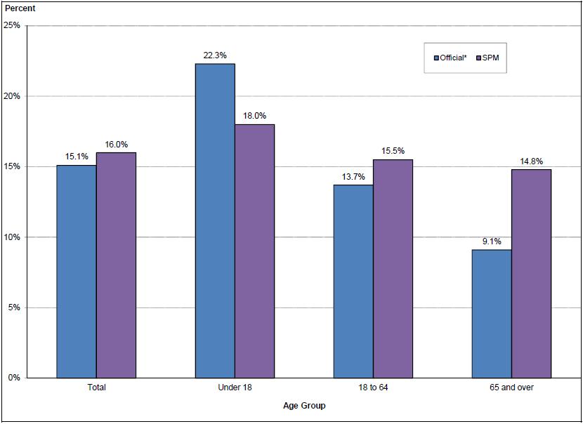
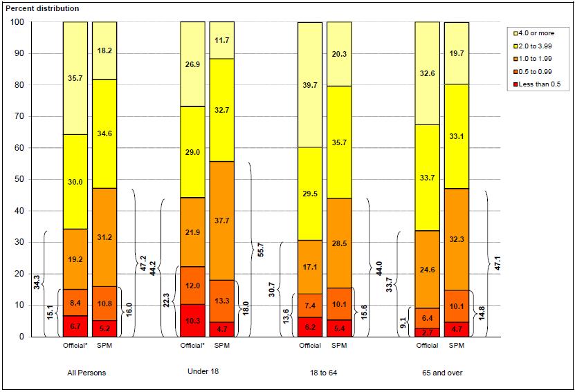
The SPM yields a very different impression of the incidence of poverty with respect to age than that portrayed by the "official" measure. Figure 9 compares poverty rates by age group under the SPM and the "official" measure in 2012. The poverty rate for adults ages 18 to 64 is somewhat higher under the SPM than under the "official" measure (15.5% compared to 13.7%). The figure shows that the poverty rate for children (under age 18) is lower under the SPM than under the "official" measure (18.0% compared to 22.3%). In contrast, the poverty rate among persons age 65 and over is much higher under the SPM than under the "official" measure (14.8% compared to 9.1%). Although the child poverty rate is lower under the SPM than under the "official" measure, and the aged poverty rate is considerably higher, the incidence of poverty among children still exceeds that of the aged under the SPM, as it did under the "official" measure. The SPM paints a much different picture of poverty among the aged than that conveyed by the "official" measure. As will be shown later, much of the difference between the aged poverty rate measured under the SPM compared to the "official" measure is attributable to the effect of medical expenses on the disposable income among aged units to meet basic needs represented by the SPM resource thresholds.
Figure 9. Poverty Rates Under the "Official"* and Research Supplemental Poverty Measures, by Age: 2012
(Percent poor)

Source: Figure prepared by the Congressional Research Service (CRS), based on Kathleen Short, The Research SUPPLEMENTAL POVERTY MEASURE: 2012, U.S. Census Bureau, P60-247, Washington, DC, November 2013 http://www.census.gov/prod/2013pubs/p60-247.pdf.
* Differs from published "official" poverty rates as unrelated individuals under age 15 are included in the universe.
Poverty by Type of Economic Unit
As noted above, the SPM expands the definition of the economic unit considered for poverty measurement purposes over that used under the "official" poverty measure. The "official" poverty measure groups all co-residing household members related by marriage, birth, or adoption as sharing resources for purposes of poverty determination. Unrelated individuals, whether living alone as a single person household or with other unrelated members, are treated as separate economic units under the "official" poverty measure. The "official" measure also excludes unrelated children under age 15 from the universe for poverty determination. As noted earlier, the "adjusted official" poverty measure presented in this section of the report includes unrelated children, resulting in a 15.1% poverty rate as opposed to the published rate of 15.0% in 2012.
The SPM expands the economic unit used for poverty determination beyond that used by the "official" measure. |25| The SPM assesses the relationship of unrelated household members to others in the household to determine whether they will be joined with others to construct expanded economic units. For example, the SPM combines unrelated co-residing household members age 14 and older who are not married and who identify each other as boyfriend, girlfriend, or partner as cohabiting partners. Cohabiting partners, as well as any of their coresident family members, are combined as an economic unit under the SPM. The SPM also combines unmarried co-residing parents of a child living in the household as an economic unit, even if the parents do not identify as a cohabiting couple. Any unrelated children who are under age 15 and are not foster children are assigned to the householder's economic unit, as are foster children under the age of 22. Additionally, the SPM combines children over age 18 living in a household with a parent, and any younger children of the parent, as an economic unit. Under the "official" poverty measure, a child age 18 and over is treated as an unrelated individual, and the child's parent is also treated as an unrelated individual if no other family members are present, or as an unrelated subfamily head if a spouse or other children (under age 18) are also residing in the household.
In 2012, an estimated 27.9 million persons, 9.0% of the 311.1 million persons represented in the CPS/ASEC, were classified as either joining an economic unit or having members added to their economic unit under the SPM measure, compared to how they would have been classified under the "official" measure's economic unit definition. Combining the resources of these additional household members had the effect of reducing poverty under the SPM measure, compared to the "official" measure, in 2012.
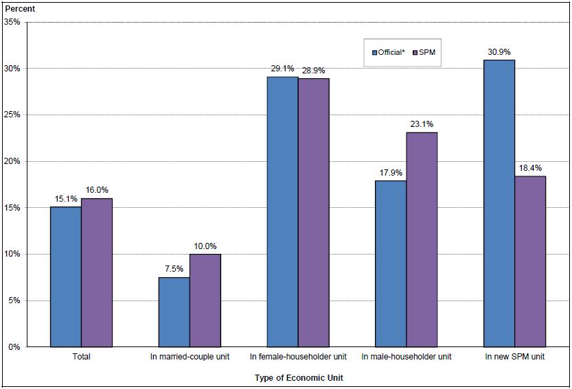
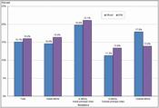
Figure 10 shows poverty rates in 2012 by type of economic unit. Persons identified as being in a married-couple unit, or in female- or male-householder units, are persons in those economic units whose members remained unchanged under the SPM compared to the "official" poverty measure. Persons who were added to an economic unit, or were part of an economic unit that had members added to it under the SPM definition, are labeled as being in a "new SPM unit." The figure shows that poverty rates for persons in married-couple units, and in male-householder units, are higher under the SPM than under the "official" poverty measure (10.0% versus 7.5% for persons in married-couple units, and 23.1% versus 17.9% for persons in male-householder units). Poverty rates for persons living in female-householder units did not statistically differ from one another, with about 3 out of 10 persons in such units considered poor under either measure. In contrast, poverty among persons who were members of "new SPM units" fell by over one-third, from 30.9% under the "official" measure to 18.4% under the SPM.
Figure 10. Poverty Rates Under the "Official"* and Research Supplemental Poverty Measures, by Type of Economic Unit: 2012
(Percent Poor)
Source: Figure prepared by the Congressional Research Service (CRS), based on Kathleen Short, The Research SUPPLEMENTAL POVERTY MEASURE: 2012, U.S. Census Bureau, P60-247, Washington, DC, November 2013 http://www.census.gov/prod/2013pubs/p60-247.pdf.
* Differs from published "official" poverty rates as unrelated individuals under age 15 are included in the universe.
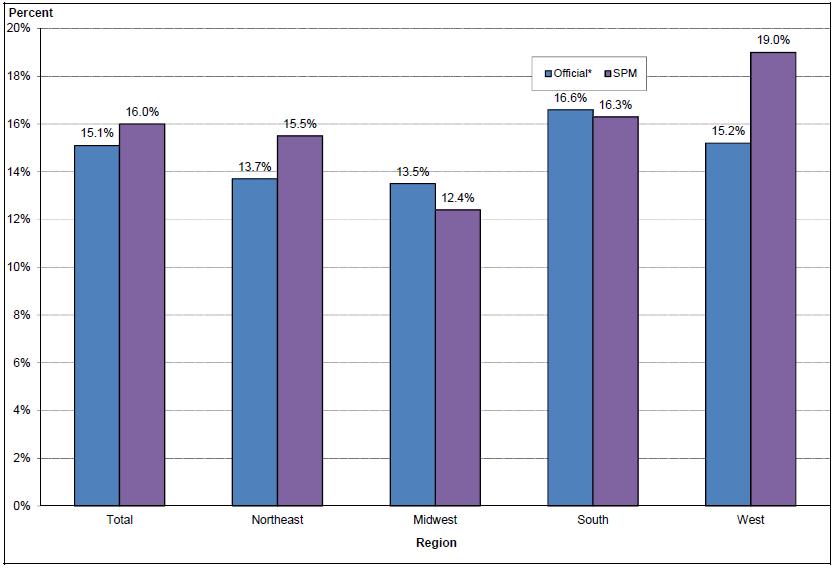
Figure 11 compares poverty rates in 2012 under the SPM with the "official" measure by Census region. The figure shows that poverty rates in the West are considerably higher (25% higher) under the SPM (19.0%) than under the "official" measure (15.2%). Poverty rates are about 13% higher in the Northeast under the SPM (15.5%) compared to the "official" measure (13.1%). Poverty rates in the Midwest are lower under the SPM than under the "official" measure, and in the South, essentially equal. The differences in poverty rates within and between regions based on the SPM compared to the "official" measure are most directly due to the SPM's geographic price adjustments to poverty thresholds for differences in the cost of housing in metropolitan and nonmetropolitan areas across states. The cost of housing tends to be higher in the West and Northeast, causing their poverty rates to rise under the SPM relative to the "official" measure and relative to the South and Midwest, where housing tends to be less expensive.
Figure 11. Poverty Rates Under the "Official"* and Research Supplemental Poverty Measures, by Region: 2012
(Percent Poor)

Source: Figure prepared by the Congressional Research Service (CRS), based on Kathleen Short, The Research SUPPLEMENTAL POVERTY MEASURE: 2012, U.S. Census Bureau, P60-247, Washington, DC, November 2013 http://www.census.gov/prod/2013pubs/p60-247.pdf.
* Differs from published "official" poverty rates as unrelated individuals under age 15 are included in the universe.
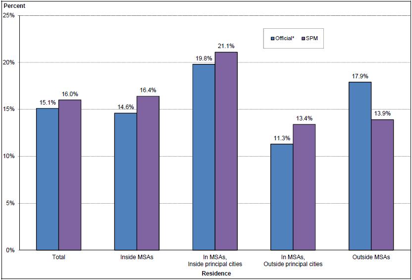
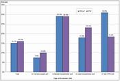
Figure 12 depicts poverty rates by residence in metropolitan (principal city, and outside principal city [i.e., "suburban"]) and nonmetropolitan areas in 2012. |26| The fi gure shows that under the SPM, the poverty rate for persons living in Metropolitan Statistical Areas (MSAs) (16.4%) is somewhat higher than under the "official" measure (14.6%), whereas for persons living outside MSAs, the poverty rate is lower under the SPM (13.9%) than under the "official" measure (17.9%). Again, this most likely reflects differences in the cost of housing between MSAs and non-MSAs. Within MSAs, poverty rates are higher for persons living within principal cities under both measures than for people living outside them in "suburban" or "ex-urban" areas.
Figure 12. Poverty Rates Under the "Official"* and Research Supplemental Poverty Measures, by Residence: 2012
(Percent Poor)
Source: Figure prepared by the Congressional Research Service (CRS), based on Kathleen Short, The Research SUPPLEMENTAL POVERTY MEASURE: 2012, U.S. Census Bureau, P60-247, Washington, DC, November 2013 http://www.census.gov/prod/2013pubs/p60-247.pdf.
* Differs from published "official" poverty rates as unrelated individuals under age 15 are included in the universe.
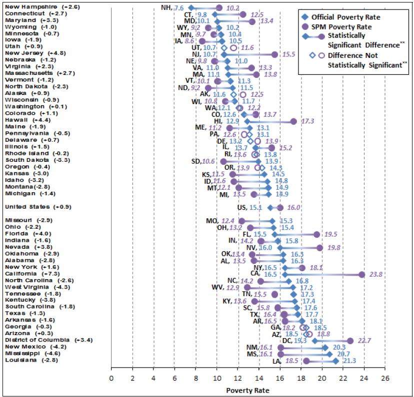
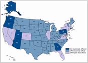
Figure 13 depicts states according to whether the state's SPM poverty rate statistically differs from its "official" poverty rate. |27| Estimates are based on three-year (2010 to 2012) averages of CPS/ASEC data. Three years of data are combined in order to improve the statistical reliability of CPS/ASEC estimates at the state level. The figure shows that 13 states (California, Colorado, Connecticut, Florida, Hawaii, Illinois, Maryland, Massachusetts, New Hampshire, New Jersey, New York, Nevada, and Virginia) and the District of Columbia had higher poverty rates under the SPM than under the "official" measure. Among the 13 states with higher SPM poverty rates than their respective "official" poverty rate, only Colorado, Illinois, and Nevada were inland, and with the exception of Florida and Virginia, none were in the South. The figure shows that the SPM poverty rate was not statistically different than the "official" poverty rate in nine states (Alaska, Arizona, Delaware, Georgia, Oregon, Pennsylvania, Rhode Island, Utah, and Washington). Among the 28 remaining states in which their SPM poverty rates were lower than their respective "official" poverty rates, nearly all (with Maine being the exception) were either in the South, or inland.
Figure 13. Difference in Poverty Rates by State Using the "Official"* Measure and the SPM: Three-Year Average 2010-2012
Source: Figure prepared by the Congressional Research Service (CRS), based on Kathleen Short, The Research SUPPLEMENTAL POVERTY MEASURE: 2012, U.S. Census Bureau, P60-247, Washington, DC, November 2013 http://www.census.gov/prod/2013pubs/p60-247.pdf.
Notes: Within state difference between official and SPM poverty rates determined at a 90% statistical confidence level.
* Differs from published "official" poverty rates as unrelated individuals under age 15 are included in the universe.
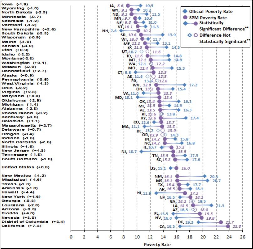
Figure 14 and Figure 15 depict poverty rates by state under the official poverty measure and the SPM based on three years of CPS/ASEC data. Estimates are based on three-year (2010 to 2012) averages to improve the statistical reliability of estimates attainable from CPS/ASEC data at the state level. The two figures differ only in terms of the order in which states are sorted. In Figure 14, states are sorted from lowest to highest based on their respective "official" poverty rate point estimates, whereas in Figure 15 states are sorted from lowest to highest based on their respective SPM poverty rate point estimates. In neither figure are precise rankings of states possible because of the depicted margin of error around each state's estimate. Within a state, a statistically significant difference |28| between a state's official poverty rate and its SPM poverty rate is signified by solid-filled markers, indicating the point estimate under each measure, and a line connecting them, indicating the estimated difference (which is also shown in parentheses after each state name). The figures show the magnitude of the difference among the 13 states and the District of Columbia that had statistically significant higher poverty rates under the SPM than under the "official" measure, as well as for the 28 states in which the state's SPM rate was lower than its "official" poverty rate and the 9 states in which the incidence of poverty under the two measures did not differ statistically.
Differences in state poverty rates based on the SPM compared to the "official" measure may be due to a variety of factors. Geographic adjustments to SPM poverty income thresholds to account for differences in housing costs tend to result in higher poverty rates in areas with higher-priced housing than in areas with lower-priced housing. The mix of housing tenure (e.g., owner occupied, with or without a mortgage, renter occupied) may account for some of the difference between "official" and SPM poverty rates, within and between areas. Similarly, taxes may differ among areas. Also, populations may differ across areas in terms of household composition (e.g., share of households with cohabiting partners). The composition of the population based on age, or health insurance status, may also affect the incidence of SPM poverty relative to "official" poverty within and between geographic areas, by affecting medical out of pocket spending (MOOP), which is considered by SPM in estimating poverty.
Among the states with a statistically significant increase in poverty under the SPM, California's poverty rate increased by more than any other state's, increasing from 16.5% under the "official" measure to 23.8% under the SPM, or 7.3 percentage points. Under the "official" measure, California's poverty rate was substantially above the U.S. rate (15.1%), but under the SPM, California's poverty rate is estimated as the highest in the nation.
Other states with comparatively large increases in their poverty rates (in the four percentage point range) under the SPM compared to the "official" measure include Hawaii (an increase from 12.0% to 17.3%), Florida (a 15.5% to 19.5% increase), and New Jersey (a 10.7% to 15.5% increase).
Three states had decreases in their SPM poverty rate compared to their "official" rate in the four percentage point range. Mississippi and New Mexico, among the states with the highest "official" poverty (20.7% and 20.3%, respectively), both have an estimated SPM poverty rate of 16.1%-- just about equal to the U.S. SPM rate (16.0%). West Virginia's "official" poverty rate (17.2%) is well above the "official" U.S. rate (15.1%), but its SPM rate (12.9%) falls well below the U.S. SPM rate (16.0%).
Figure 14. Poverty Rates by State Using the "Official"* Measure and the SPM:
Three-Year Average 2010-2012
(States Ranked in Ascending Order by Official Poverty Rate; Percentage Point Difference in Parentheses)
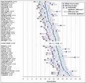
Source: Figure prepared by the Congressional Research Service (CRS), based on Kathleen Short, The Research SUPPLEMENTAL POVERTY MEASURE: 2012, U.S. Census Bureau, P60-247, Washington, DC, November 2013 http://www.census.gov/prod/2013pubs/p60-247.pdf.
* Differs from published "official" poverty rates as unrelated individuals under age 15 are included in the universe.
** Within state difference between official and SPM poverty rates determined at a 90% statistical confidence level.
Figure 15. Poverty Rates by State Using the "Official"* Measure and the SPM: Three-Year Average 2010-2012
(States Ranked in Ascending Order by SPM Poverty Rate; Percentage Point Difference in Parentheses)
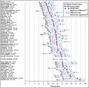
Source: Figure prepared by the Congressional Research Service (CRS), based on Kathleen Short, The Research SUPPLEMENTAL POVERTY MEASURE: 2012, U.S. Census Bureau, P60-247, Washington, DC, November 2013 http://www.census.gov/prod/2013pubs/p60-247.pdf
* Differs from published "official" poverty rates as unrelated individuals under age 15 are included in the universe.
** Within state difference between official and SPM poverty rates determined at a 90% statistical confidence level.
Marginal Effects of Counting Specified Resources and Expenses on Poverty Under the SPM
Figure 16 focuses strictly on the SPM, examining the marginal effects on poverty rates attributable to the inclusion of each selected income/resource or expenditure element on the measure. The marginal effects of each element on the SPM are displayed by age group. Elements that marginally contribute resources, and thereby have a poverty reducing effect when included in the SPM, are ranked from left to right in terms of their effect on poverty reduction among all persons. Similarly, expenditure elements, which are subtracted from resources and thereby marginally increase poverty as measured by the SPM, are ranked from left to right by their marginal poverty increasing effects on all persons.
The figure shows, for example, that the EITC has a greater poverty reducing effect than any of the other depicted resource elements. Overall, the EITC lowers the SPM poverty rate for all persons by 3.0 percentage points. The EITC is followed by SNAP benefits (1.6 percentage point reduction), housing subsidies (0.9 percentage point reduction), school lunch (0.4 percentage point reduction), and WIC and LIHEAP (each with a 0.1 percentage point reduction).
In contrast, on the expenditure side, child support paid to members outside the household has a relatively small effect on increasing the overall poverty rate. Federal income taxes before considering refundable credits, such as the EITC (counted on the resource side), result in an increase in overall poverty of 0.4 percentage points. FICA payroll taxes have a larger effect on marginal poverty (1.6 percentage point increase) than federal income taxes, as do work expenses (1.9 percentage points). Among all of the expense elements presented, medical out of pocket expenses (MOOP) contribute to the largest increase in poverty (3.4 percentage point increase for all persons).
Among the three age groups, the additional resources included in the SPM have a greater effect on reducing poverty among children (persons under age 18) and poverty among working age adults (ages 18 to 64) than on the aged (age 65 and older), with the exception of housing subsidies, which reduce the aged poverty rate by about the same amount as that of children. The EITC has a greater effect of reducing poverty among children (6.7 percentage point reduction) than any of the other added SPM resources.
On the expenditure side, FICA payroll taxes and work expenses have a greater effect on increasing poverty among children (due to a working parent) and non-aged adults than on the aged, who are less likely to be in the labor force and incur work-related taxes and expenses. Notably, under the SPM, MOOP expenses contribute to a substantial increase in poverty among the aged, contributing to a 6.4 percentage point increase in their poverty rate.
The relative distribution of additional resources and expenses in the SPM by age group helps to explain why poverty among children is lower under the SPM than it is under the "official" measure, whereas it is considerably higher for the aged.
Figure 16. Percentage Point Change in Poverty Rates Attributable to Selected Income and Expenditure Elements Under the Research Supplemental Poverty Measure, by Age Group: 2012
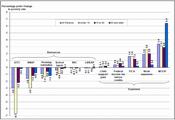
Source: Figure prepared by the Congressional Research Service (CRS), based on Kathleen Short, The Research SUPPLEMENTAL POVERTY MEASURE: 2012, U.S. Census Bureau, P60-247, Washington, DC, November 2013 http://www.census.gov/prod/2013pubs/p60-247.pdf.
Distribution of the Population by Ratio of Income/Resources Relative to Poverty
Figure 17 shows the distribution of the population by age group according to the degree to which their income and resources fall below or above poverty under the "official" and SPM definitions. The figure breaks out the poor population, depicted by brackets, into the share whose income and resources fall below half of their respective poverty lines (a classification sometimes referred to as "deep poverty") and the remainder. Others are categorized by the extent to which their income/resources exceed poverty under the two definitions, with those who fall below twice the poverty line also demarcated by brackets.
The figure shows, for example, that the share of children in "deep poverty" under the SPM is considerably lower than under the "official" measure (4.7% compared to 10.3%). As shown earlier, the SPM child poverty rate (18.0%) is lower than the "official" rate (22.3%). However, under the SPM, a much greater share of children live in "families" with income/resources between one and two times the poverty line than under the "official" measure (33.7% and 21.9%). Altogether, well over half of the children live in "families" having income/resources below twice the poverty line under the SPM (55.7%) compared to over two-fifths (44.2%) under the "official" measure. Thus, while the SPM appears to result in fewer children being counted as poor than under the "official" measure, under the SPM a greater share than under the "official" measure are concentrated at income levels just above poverty.
Among persons age 65 and over, a greater share are poor under the SPM than under the "official" measure, as shown earlier (14.8% compared to 9.1%), and a greater share are in "deep poverty" under the SPM (4.7%) than under the "official" measure (2.7%). In contrast to the "official" measure, under which about one-third (32.3%) of the aged have income below 200% of poverty, almost half (47.1%) have income/resources below that level under the SPM.
Figure 17. Distribution of the Population by Income/Resources to Poverty Ratios Under the "Official"* and Research Supplemental Poverty Measures, by Age Group: 2012
(Percent distribution)
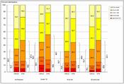
Source: Figure prepared by the Congressional Research Service (CRS), based on Kathleen Short, The Research SUPPLEMENTAL POVERTY MEASURE: 2012, U.S. Census Bureau, P60-247, Washington, DC, November 2013 http://www.census.gov/prod/2013pubsZp60-247.pdf.
* Differs from published "official" poverty rates as unrelated individuals under age 15 are included in the universe.
As a research measure, the SPM offers potential for improved insight leading to better understanding of the nature and circumstances of those deemed to be among the nation's most economically and socially vulnerable. The SPM offers the means to better assess the performance of the economy, government policies, and programs with regard to the population's ability to secure sufficient income/resources to be able to meet basic expenditures for food, clothing, shelter, and utilities (plus "a little bit more").
The SPM counts considerably more elderly as poor than does the "official" measure. Medical expenses appear to be the driving factor in increasing poverty among the elderly under the SPM (see Figure 16). While not negating the improvement in the poverty status of the aged over the years, based on the "official" measure (see Figure 2), the SPM points more directly to the economic vulnerability of the aged, based not on income/resources alone, but rather, medical expenses competing for income that might otherwise be used to meet basic needs (i.e., FCSU plus "a little bit more"). Rising medical costs in society overall and individuals' personal health and insurance statuses pose potential economic risk to the aged being able to meet basic needs, as captured by FCSU-based poverty thresholds. The SPM provides additional insight that poverty reduction among the elderly depends not only on improving income, but also on their ability to reduce exposure to high medical expenses through "affordable" insurance. Rising medical costs in society also place the aged at increased risk of poverty under the SPM. It is worth noting that the SPM does not consider financial assets, other than interest, dividends, and annuity income from those assets, nor non-liquid assets (e.g., home equity) in determining poverty status. The SPM therefore does not address the means or extent to which the aged might tap those assets to meet medical or other needs.
The SPM results in fewer children being counted as poor than under the "official" measure. Still, the incidence of child poverty under the SPM, as under the "official" measure, exceeds that of the aged, but by a much slimmer margin (see Figure 9). Work-based supports, which both encourage work and help to offset the costs of going to work, appear be especially important to families with children, as captured by the SPM. The EITC, not counted under the "official" measure, significantly reduces child poverty as measured by the SPM, helping to offset taxes and work-related expenses working families with children incur (also captured by the SPM, but not under the "official" measure) (see Figure 16). The lack of safe, reliable, and affordable child care may limit parents' attachment to the labor force, contributing to poverty by reducing earnings that parents might otherwise secure. The SPM recognizes child care as a necessary expense many families face in their decisions relating to work by subtracting work-related child care expenses from income/resources that might otherwise go to meeting basic needs (i.e., FCSU plus "a little bit more"). As a consequence, the SPM should be sensitive to measuring the effects of child care programs and policies on child care affordability and poverty. The SPM captures the policy effects of assisting the poor through the provision of in-kind benefits, as opposed to just cash, whereas the "official" measure does not. For example, SNAP benefits, not captured under the "official" poverty measure, appear to have a sizeable effect in reducing child poverty under the SPM. Additionally, the expansion of the economic unit under the SPM to include cohabiting partners and their relatives may also contribute to lower child poverty rates under the SPM than under the "official" poverty measure, which is based on family ties defined by blood, marriage, and adoption.
[Source: By Thomas Gabe, Congressional Research Service, RL33069, Washington D.C., 13Nov13. Thomas Gabe is a Specialist in Social Policy.]
Appendix A. U.S. Poverty Statistics: 1959-2012
Table A-1. Poverty Rates (Percent Poor) for Selected Groups, 1959-2012
Year All
personsRelated Children Under Age 18a Adults Race/Ethnicityb--All Ages Total In Female-
Headed
FamiliesIn All
Other
FamiliesAges
18-64Age 65+ Whiteb White Non-
HispanicbBlackb Hispanicb Asianb 2012 15.0 21.3 47.2 12.5 13.7 9.1 12.7b 9.7b 27.2b 25.6 11.7b 2011 15.0 21.4 47.6 12.1 13.7 8.7 12.8b 9.8b 27.6b 25.3 12.3b 2010r 15.1 21.5 46.6 12.9 13.8 8.9 13.0b 9.9b 27.4b 26.5 12.2b 2009 14.3 20.1 44.4 12.3 12.9 8.9 12.3b 9.4b 25.8b 25.3 12.5b 2008 13.2 18.5 43.5 10.7 11.7 9.7 11.2b 8.6b 24.7b 23.2 11.8b 2007 12.5 17.6 43.0 9.5 10.9 9.7 10.5b 8.2b 24.5b 21.5 10.2b 2006 12.3 16.9 42.1 9.0 10.8 9.4 10.3b 8.2b 24.3b 20.6 10.3b 2005 12.6 17.7 42.8 9.3 11.1 10.1 10.6b 8.3b 24.9b 21.8 11.1b 2004r 12.7 17.3 41.9 9.7 11.3 9.8 10.8b 8.7b 24.7b 21.9 9.8b 2003 12.5 17.2 41.8 9.6 10.8 10.2 10.5b 8.2b 24.4b 22.5 11.8b 2002 12.1 16.3 39.6 9.2 10.6 10.4 10.2b 8.0b 24.1b 21.8 10.1b 2001 11.7 15.8 39.3 8.8 10.1 10.1 9.9 7.8 22.7 21.4 n/a 2000r 11.3 15.6 40.1 8.6 9.6 9.9 9.5 7.4 22.5 21.5 n/a 1999 11.8 16.3 41.9 9.0 10.0 9.7 9.8 7.7 23.6 22.8 n/a 1998 12.7 18.3 46.1 9.7 10.5 10.5 10.5 8.2 26.1 25.6 n/a 1997 13.3 19.2 49.0 10.2 10.9 10.5 11.0 8.6 26.5 27.1 n/a 1996 13.7 19.8 49.3 10.9 11.3 10.8 11.2 8.6 28.4 29.4 n/a 1995 13.8 20.2 50.3 10.7 11.4 10.5 11.2 8.5 29.3 30.3 n/a 1994 14.5 21.2 52.9 11.7 11.9 11.7 11.7 9.4 30.6 30.7 n/a 1993 15.1 22.0 53.7 12.4 12.4 12.2 12.2 9.9 33.1 30.6 n/a 1992r 14.8 21.6 54.6 11.8 11.9 12.9 11.9 9.6 33.4 29.6 n/a 1991r 14.2 21.1 55.5 11.1 11.4 12.4 11.3 9.4 32.7 28.7 n/a 1990 13.5 19.9 53.4 10.7 10.7 12.2 10.7 8.8 31.9 28.1 n/a 1989 12.8 19.0 51.1 10.4 10.2 11.4 10.0 8.3 30.7 26.2 n/a 1988r 13.0 19.0 52.9 10.0 10.5 12.0 10.1 8.4 31.3 26.7 n/a 1987r 13.4 19.7 54.7 10.9 10.6 12.5 10.4 8.7 32.4 28.0 n/a 1986 13.6 19.8 54.4 10.8 10.8 12.4 11.0 9.4 31.1 27.3 n/a 1985 14.0 20.1 53.6 11.7 11.3 12.6 11.4 9.7 31.3 29.0 n/a 1984 14.4 21.0 54.0 12.5 11.7 12.4 11.5 10.0 33.8 28.4 n/a 1983 15.2 21.8 55.5 13.5 12.4 13.8 12.2 10.8 35.7 28.1 n/a 1982 15.0 21.3 56.0 13.0 12.0 14.6 12.0 10.6 35.6 29.9 n/a 1981 14.0 19.5 52.3 11.6 11.1 15.3 11.1 9.9 34.2 26.5 n/a 1980 13.0 17.9 50.8 10.4 10.1 15.7 10.2 9.1 32.5 25.7 n/a 1979 11.7 16.0 48.6 8.5 8.9 15.2 9.0 8.1 31.0 21.8 n/a 1978 11.4 15.7 50.6 7.9 8.7 14.0 8.7 7.9 30.6 21.6 n/a 1977 11.6 16.0 50.3 8.5 8.8 14.1 8.9 8.0 31.3 22.4 n/a 1976 11.8 15.8 52.0 8.5 9.0 15.0 9.1 8.1 31.1 24.7 n/a 1975 12.3 16.8 52.7 9.8 9.2 15.3 9.7 8.6 31.3 26.9 n/a 1974 11.2 15.1 51.5 8.3 8.3 14.6 8.6 7.7 30.3 23.0 n/a 1973 11.1 14.2 52.1 7.6 8.3 16.3 8.4 7.5 31.4 21.9 n/a 1972 11.9 14.9 53.1 8.6 8.8 18.6 9.0 n/a 33.3 n/a n/a 1971 12.5 15.1 53.1 9.3 9.3 21.6 9.9 n/a 32.5 n/a n/a 1970 12.6 14.9 53.0 9.2 9.0 24.6 9.9 n/a 33.5 n/a n/a 1969 12.1 13.8 24.4 8.6 8.7 25.3 9.5 n/a 32.2 n/a n/a 1968 12.8 15.3 55.2 10.2 9.0 25.0 10.0 n/a 34.7 n/a n/a 1967 14.2 16.3 54.3 11.5 10.0 29.5 11.0 n/a 39.3 n/a n/a 1966 14.7 17.4 58.2 12.6 10.5 28.5 11.3 n/a 41.8 n/a n/a 1959 22.4 26.9 72.2 22.4 17.0 35.2 18.1 n/a 55.1 n/a n/a Source: Prepared by the Congressional Research Service using U.S. Bureau of the Census data based on the "official" measure of poverty.
Notes: r = revised estimates. n/a = not available.
a. Beginning in 1979, restricted to children in primary families only. Before 1979, includes children in unrelated subfamilies.
b. Beginning in 2002, CPS respondents could identify themselves as being of more than one race. Consequently, racial data for 2002 and after are not comparable to earlier years. Here, in 2002 and after, the term white means of white race alone, the term black means of black race alone, and the term Asian means Asian alone. Hispanics, who may be of any race, are included among whites and blacks unless otherwise noted.
Appendix B. Metropolitan Area Poverty Estimates
Table B-1. Metropolitan Area Poverty: 2012
Metropolitan Area Total
PopulationNumber Poor Poverty Rate (Percent Poor) Estimate Margin of Errora Poverty Rate Margin of Errora Difference 2011 vs.
2010 Poverty RatebRankc Abilene, TX 156,020 31,991 +/-4,101 20.5% +/-2.6% 3.6% ▲ 61 Akron, OH 687,031 107,952 +/-7,892 15.7% +/-1.1% -0.9% 205 Albany, GA 148,869 40,011 +/-4,170 26.9% +/-2.8% -1.5% 8 Albany-Schenectady-Troy, NY 843,802 93,228 +/-6,350 11.0% +/-0.8% -0.4% 335 Albuquerque, NM 887,938 164,484 +/-9,170 18.5% +/-1.0% -1.9% ▼ 107 Alexandria, LA 146,869 32,184 +/-4,402 21.9% +/-3.0% -1.3% 42 Allentown-Bethlehem-Easton, PA-NJ 804,602 84,127 +/-6,553 10.5% +/-0.8% -1.4% ▼ 346 Altoona, PA 124,522 15,955 +/-2,286 12.8% +/-1.8% -1.5% 297 Amarillo, TX 245,710 43,548 +/-5,530 17.7% +/-2.2% 2.2% 133 Ames, IA 82,352 17,880 +/-2,472 21.7% +/-3.0% -2.3% 44 Anchorage, AK 384,749 33,353 +/-4,104 8.7% +/-1.1% -0.1% 361 Anderson, IN 123,288 18,763 +/-2,891 15.2% +/-2.3% -4.3% ▼ 224 Anderson, SC 186,924 33,612 +/-4,647 18.0% +/-2.5% 3.2% 124 Ann Arbor, MI 334,662 55,178 +/-5,538 16.5% +/-1.6% -0.5% 171 Anniston-Oxford, AL 114,001 25,270 +/-3,403 22.2% +/-3.0% 1.0% 38 Appleton, WI 225,045 18,885 +/-2,630 8.4% +/-1.2% 1.0% 362 Asheville, NC 422,827 66,980 +/-5,197 15.8% +/-1.2% -1.1% 201 Athens-Clarke County, GA 183,413 44,991 +/-3,612 24.5% +/-1.9% -5.4% ▼ 16 Atlanta-Sandy Springs-Marietta, GA 5,352,236 887,901 +/-29,846 16.6% +/-0.6% -0.2% 166 Atlantic City-Hammonton, NJ 269,061 39,381 +/-5,807 14.6% +/-2.2% 1.2% 246 Auburn-Opelika, AL 141, 938 34,970 +/-3,720 24.6% +/-2.6% 1.7% 15 Augusta-Richmond County, GA-SC 553,981 112,218 +/-8,963 20.3% +/-1.6% 1.3% 66 Austin-Round Rock-San Marcos, TX 1,795,080 278,461 +/-16,086 15.5% +/-0.9% 0.3% 211 Bakersfield-Delano, CA 825,020 196,625 +/-13,837 23.8% +/-1.7% -0.7% 23 Baltimore-Towson, MD 2,685,159 303,704 +/-14,893 11.3% +/-0.6% -0.3% 329 Bangor, ME 146,973 26,664 +/-3,346 18.1% +/-2.3% 0.6% 118 Barnstable Town, MA 212,878 21,947 +/-3,653 10.3% +/-1.7% 1.1% 350 Baton Rouge, LA 791,990 148,176 +/-10,354 18.7% +/-1.3% 1.1% 103 Battle Creek, MI 131,723 23,569 +/-3,069 17.9% +/-2.3% -1.7% 129 Bay City, MI 105,729 13,622 +/-2,199 12.9% +/-2.1% 0.4% 293 Beaumont-Port Arthur, TX 371,641 71,066 +/-6,392 19.1% +/-1.7% 1.6% 95 Bellingham, WA 199,626 33,039 +/-4,080 16.6% +/-2.0% 0.9% 169 Bend, OR 161,035 27,003 +/-5,184 16.8% +/-3.2% 3.5% 163 Billings, MT 157,398 19,325 +/-2,698 12.3% +/-1.7% -0.5% 307 Binghamton, NY 238,176 36,879 +/-3,933 15.5% +/-1.6% -0.6% 213 Birmingham-Hoover, AL 1,114,744 186,891 +/-11,466 16.8% +/-1.0% 0.2% 164 Bismarck, ND 110,290 7,266 +/-1,572 6.6% +/-1.4% -2.2% 365 Blacksburg-Christiansburg-Radford, VA 152,492 36,188 +/-3,820 23.7% +/-2.4% 2.4% 24 Bloomington, IN 180,522 41,518 +/-4,489 23.0% +/-2.5% 1.2% 30 Bloomington-Normal, IL 163,412 25,664 +/-2,990 15.7% +/-1.8% -0.2% 206 Boise City-Nampa, ID 624,906 96,368 +/-10,276 15.4% +/-1.6% -0.8% 217 Boston-Cambridge-Quincy, MA-NH 4,486,468 479,126 +/-15,238 10.7% +/-0.3% 0.0% 343 Boulder, CO 295,728 42,978 +/-4,392 14.5% +/-1.5% 0.5% 252 Bowling Green, KY 121,147 23,918 +/-3,162 19.7% +/-2.6% 1.3% 86 Bremerton-Silverdale, WA 246,659 27,164 +/-4,015 11.0% +/-1.6% 0.3% 336 Bridgeport-Stamford-Norwalk, CT 915,803 81,629 +/-7,143 8.9% +/-0.8% -0.5% 358 Brownsville-Harlingen, TX 411,003 148,267 +/-9,666 36.1% +/-2.3% 2.0% 1 Brunswick, GA 108,902 20,221 +/-3,440 18.6% +/-3.1% 0.1% 105 Buffalo-Niagara Falls, NY 1,104,704 157,407 +/-8,287 14.2% +/-0.7% -0.5% 263 Burlington, NC 150,l97 30,525 +/-3,985 20.3% +/-2.7% 1.8% 64 Burlington-South Burlington, VT 202,994 22,433 +/-2,554 11.1% +/-1.3% 0.0% 334 Canton-Massillon, OH 393,938 57,474 +/-4,951 14.6% +/-1.3% -1.9% 250 Cape Coral-Fort Myers, FL 636,067 97,210 +/-7,188 15.3% +/-1.1% -0.1% 221 Cape Girardeau-Jackson, MO-IL 92,459 16,386 +/-2,696 17.7% +/-2.9% -0.7% 134 Carson City, NV 52,680 8987 +/-2,353 17.1% +/-4.5% 3.6% 153 Casper, WY 76,446 9,816 +/-1,839 12.8% +/-2.4% 1.7% 295 Cedar Rapids, IA 254,225 24,150 +/-3,246 9.5% +/-1.3% -0.9% 355 Champaign-Urbana, IL 217,140 42,982 +/-4,172 19.8% +/-1.9% -3.0% ▼ 84 Charleston, WV 300,542 45,089 +/-4,874 15.0% +/-1.6% -3.2% ▼ 236 Charleston-North Charleston-Summerville, SC 679,648 103,056 +/-7,728 15.2% +/-1.1% -1.8% 225 Charlotte-Gastonia-Rock Hill, NC-SC 1,801,914 272,027 +/-12,223 15.1% +/-0.7% -0.6% 231 Charlottesville, VA 193,616 26,922 +/-4,417 13.9% +/-2.3% 0.9% 269 Chattanooga, TN-GA 524,863 83,083 +/-7,256 15.8% +/-1.4% -1.8% 202 Cheyenne, WY 91,949 9,822 +/-2,954 14.5% +/-3.2% 1.6% 342 Chicago-Joliet-Naperville, IL-IN-WI 9,372,358 1,362,635 +/-30,184 10.7% +/-0.3% -0.2% 251 Chico, CA 216,391 47,693 +/-5,041 22.0% +/-2.3% -1.0% 40 Cincinnati-Middletown, OH-KY-IN 2,100,460 313,902 +/-13,545 14.9% +/-0.6% 0.7% 238 Clarksville, TN-KY 277,225 53,501 +/-6,208 19.3% +/-2.2% 0.9% 94 Cleveland, TN 115,747 22,933 +/-4,094 19.8% +/-3.5% -1.2% 83 Cleveland-Elyria-Mentor, OH 2,021,864 314,832 +/-11,325 15.6% +/-0.6% -0.4% 208 Coeur d'Alene, ID 140,564 16,630 +/-3,373 11.8% +/-2.4% -4.8% 320 College Station-Bryan, TX 219,226 57,006 +/-5,130 26.0% +/-2.3% -3.9% ▼ 9 Colorado Springs, CO 649,651 83,308 +/-8,024 12.8% +/-1.2% -0.1% ▼ 296 Columbia, MO 167,502 32,391 +/-3,877 19.3% +/-2.3% -1.5% 93 Columbia, SC 751,020 122,507 +/-9,448 16.3% +/-1.3% -1.3% 184 Columbus, GA-AL 291,315 54,555 +/-5,654 18.7% +/-1.9% 1.6% 102 Columbus, IN 77,948 10,107 +/-3,297 13.0% +/-4.2% -0.5% 291 Columbus, OH 1,828,401 275,385 +/-14,679 15.1% +/-0.8% -0.3% 233 Corpus Christi, TX 428,154 69,385 +/-6,938 16.2% +/-1.6% -3.8% ▼ 188 Corvallis, OR 81,776 18,961 +/-3,400 23.2% +/-4.1% -2.2% 27 Crestview-Fort Walton Beach-Destin, FL 184, 163 25,349 +/-4,122 13.8% +/-2.2% -1.1% 279 Cumberland, MD-WV 93,858 15,330 +/-2,516 16.3% +/-2.7% -2.9% 181 Dallas-Fort Worth-Arlington, TX 6,561,480 984,719 +/-23,684 15.0% +/-0.4% -0.8% ▼ 235 Dalton, GA 141,605 30,654 +/-4,636 21.6% +/-3.3% 1.7% 46 Danville, IL 77,863 14, 165 +/-2,986 18.2% +/-3.8% -1.5% 116 Danville, VA 103, 108 18,218 +/-2,893 17.7% +/-2.8% -1.4% 138 Davenport-Moline-Rock Island, IA-IL 372,959 43,774 +/-3,939 11.7% +/-1.1% -0.9% 321 Dayton, OH 815,446 137,732 +/-10,406 16.9% +/-1.3% -0.7% 158 Decatur, AL 152,271 26,929 +/-4,140 17.7% +/-2.7% 0.7% 137 Decatur, IL 106,872 24,953 +/-2,901 23.3% +/-2.7% 9.5% ▲ 26 Deltona-Daytona Beach-Ormond Beach, FL 486,465 96,125 +/-7,463 19.8% +/-1.5% 2.6% ▲ 85 Denver-Aurora-Broomfield, CO 2,608,939 332,043 +/-15,260 12.7% +/-0.6% -0.1% 299 Des Moines-West Des Moines, IA 577,570 70,870 +/-7,393 12.3% +/-1.3% 1.1% 308 Detroit-Warren-Livonia, MI 4,248,945 740,712 +/-20,248 17.4% +/-0.5% -0.6% 144 Dothan, AL 145,259 28,928 +/-2,460 19.9% +/-1.7% 1.2% 79 Dover, DE 162,155 19,330 +/-3,736 11.9% +/-2.3% -2.5% 312 Dubuque, IA 91,565 11,447 +/-2,024 12.5% +/-2.2% 3.3% ▲ 305 Duluth, MN-WI 268,927 41,082 +/-3,386 15.3% +/-1.3% -1.4% 222 Durham-Chapel Hill, NC 498,686 89,222 +/-7,518 17.9% +/-1.5% -0.5% 130 Eau Claire, WI 155,515 21,478 +/-2,737 13.8% +/-1.8% 1.4% 272 El Centro, CA 164,473 37,332 +/-5,169 22.7% +/-3.1% -4.1% 31 El Paso, TX 812,645 195,247 +/-10,809 24.0% +/-1.3% -0.6% 21 Elizabethtown, KY 116,810 17,635 +/-3,210 15.1% +/-2.7% -0.5% 230 Elkhart-Goshen, IN 195,801 30,249 +/-4,738 15.4% +/-2.4% -5.1% ▼ 215 Elmira, NY 83,915 12,243 +/-2,120 14.6% +/-2.5% -1.4% 249 Erie, PA 267,909 42,462 +/-3,860 15.8% +/-1.4% -0.6% 200 Eugene-Springfield, OR 347,917 78,203 +/-6,911 22.5% +/-2.0% 1.1% 34 Evansville, IN-KY 347,895 48,616 +/-5,690 14.0% +/-1.6% -0.3% 268 Fairbanks, AK 96,529 6,646 +/-1,813 6.9% +/-1.9% -3.5% 364 Fargo, ND-MN 208,133 22,118 +/-2,954 10.6% +/-1.4% -3.5% ▼ 344 Farmington, NM 126,992 26,324 +/-3,243 20.7% +/-2.6% 3.6% 59 Fayetteville, NC 362,499 61,869 +/-5,946 17.1% +/-1.6% -1.5% 152 Fayetteville-Springdale-Rogers, AR-MO 470,725 82,980 +/-8,224 17.6% +/-1.7% 0.4% 139 Flagstaff, AZ 127,795 33,191 +/-4,344 26.0% +/-3.4% 4.1% 10 Flint, MI 412,418 88,137 +/-6,951 21.4% +/-1.7% 0.8% 49 Florence, SC 201,858 43,134 +/-4,783 21.4% +/-2.4% -0.1% 50 Florence-Muscle Shoals, AL 144,910 27,196 +/-3,724 18.8% +/-2.6% 2.3% 101 Fond du Lac, WI 98,703 8,608 +/-1,938 8.7% +/-2.0% -0.9% 360 Fort Collins-Loveland, CO 302,392 42,316 +/-4,411 14.0% +/-1.5% -0.2% 267 Fort Smith, AR-OK 292,035 66,011 +/-5,561 22.6% +/-1.9% 2.1% 32 Fort Wayne, IN 414,634 62,557 +/-5,884 15.1% +/-1.4% -1.0% 232 Fresno, CA 930,872 264,738 +/-13,321 28.4% +/-1.4% 2.7% ▲ 5 Gadsden, AL 102,682 21,819 +/-3,915 21.2% +/-3.8% 0.3% 52 Gainesville, FL 254,375 70,552 +/-5,754 27.7% +/-2.2% 3.6% ▲ 6 Gainesville, GA 182,805 37,000 +/-5,945 20.2% +/-3.3% 2.8% 67 Glens Falls, NY 124,271 14,242 +/-2,612 11.5% +/-2.1% -3.1% 328 Goldsboro, NC 121,372 30,174 +/-4,262 24.9% +/-3.5% 1.5% 14 Grand Forks, ND-MN 93,134 16,629 +/-2,265 17.9% +/-2.4% 3.0% 132 Grand Junction, CO 144,569 23,285 +/-4,260 16.1% +/-2.9% 4.8% ▲ 192 Grand Rapids-Wyoming, MI 770,026 126,882 +/-9,164 16.5% +/-1.2% 1.8% ▲ 173 Great Falls, MT 79,862 15,919 +/-2,657 19.9% +/-3.3% 4.3% 76 Greeley, CO 255,850 37,734 +/-5,186 14.7% +/-2.0% 0.0% 242 Green Bay, WI 303,843 34,897 +/-3,993 11.5% +/-1.3% 1.2% 327 Greensboro-High Point, NC 718,572 130,400 +/-8,783 18.1% +/-1.2% 0.5% 117 Greenville, NC 185,538 45,060 +/-4,358 24.3% +/-2.3% -1.1% 19 Greenville-Mauldin-Easley, SC 630,562 111,529 +/-8,864 17.7% +/-1.4% 0.2% 136 Gulfport-Biloxi, MS 250,861 50,407 +/-6,494 20.1% +/-2.6% 1.7% 69 Hagerstown-Martinsburg, MD-WV 263,149 38,424 +/-6,225 14.6% +/-2.4% 1.0% 247 Hanford-Corcoran, CA 131,214 27,819 +/-4,294 21.2% +/-3.3% 0.7% 53 Harrisburg-Carlisle, PA 536,028 66,476 +/-6,615 12.4% +/-1.2% 1.9% ▲ 306 Harrisonburg, VA 119,527 26,436 +/-3,424 22.1% +/-2.9% 6.4% ▲ 39 Hartford-West Hartford-East Hartford, CT 1,169,356 127,371 +/-7,291 10.9% +/-0.6% -0.5% 338 Hattiesburg, MS 143,389 36,577 +/-4,869 25.5% +/-3.4% 1.2% 12 Hickory-Lenoir-Morganton, NC 355,419 71,802 +/-6,072 20.2% +/-1.7% 1.8% 68 Hinesville-Fort Stewart, GA 81,660 13,250 +/-2,842 16.2% +/-3.4% -2.7% 187 Holland-Grand Haven, MI 259,849 29,263 +/-4,634 11.3% +/-1.8% -0.8% 330 Honolulu, HI 945,975 97,754 +/-8,616 10.3% +/-0.9% 0.2% 349 Hot Springs, AR 95,247 18,951 +/-3,488 19.9% +/-3.7% -1.9% 78 Houma-Bayou Cane-Thibodaux, LA 205,153 32,847 +/-4,949 16.0% +/-2.4% -2.9% 194 Houston-Sugar Land-Baytown, TX 6,123,358 1,005,192 +/-32,475 16.4% +/-0.5% -1.0% ▼ 176 Huntington-Ashland, WV-KY-OH 277,846 50,941 +/-4,448 18.3% +/-1.6% -1.5% 112 Huntsville, AL 419,921 50,052 +/-6,323 11.9% +/-1.5% -2.1% 313 Idaho Falls, ID 132,174 18,157 +/-3,400 13.7% +/-2.6% 0.0% 277 Indianapolis-Carmel, IN 1,764,733 253,758 +/-13,144 14.4% +/-0.7% 0.3% 256 Iowa City, IA 149,364 22,596 +/-2,802 15.1% +/-1.9% -3.6% ▼ 226 Ithaca, NY 89,419 16,194 +/-2,444 18.1% +/-2.7% -2.9% 119 Jackson, MI 150,510 29,934 +/-3,371 19.9% +/-2.2% 4.6% ▲ 81 Jackson, MS 531,354 117,984 +/-8,520 22.2% +/-1.6% 3.7% ▲ 36 Jackson, TN 110,454 19,155 +/-3,275 17.3% +/-2.9% -3.3% 146 Jacksonville, FL 1,349,273 211,746 +/-12,970 15.7% +/-1.0% 0.5% 207 Jacksonville, NC 169,165 20,586 +/-4,627 12.2% +/-2.7% -3.1% 309 Janesville, WI 156,384 24,314 +/-3,399 15.5% +/-2.2% 0.5% 210 Jefferson City, MO 139,737 21,555 +/-4,364 15.4% +/-3.1% 3.1% 216 Johnson City, TN 194,031 37,682 +/-4,368 19.4% +/-2.2% -0.3% 91 Johnstown, PA 133,355 19,334 +/-1,996 14.5% +/-1.5% 0.5% 253 Jonesboro, AR 118,862 23,465 +/-2,594 19.7% +/-2.2% -2.8% 87 Joplin, MO 170,601 30,537 +/-3,179 17.9% +/-1.9% 2.4% 128 Kalamazoo-Portage, MI 321,649 58,206 +/-5,144 18.1% +/-1.6% -2.7% ▼ 120 Kankakee-Bradley, IL 108,498 19,501 +/-3,052 18.0% +/-2.8% 1.3% 125 Kansas City, MO-KS 2,028,356 261,177 +/-12,866 12.9% +/-0.6% -0.6% 294 Kennewick-Pasco-Richland, WA 263,116 38,061 +/-5,468 14.5% +/-2.1% -2.2% 254 Killeen-Temple-Fort Hood, TX 396,374 59,346 +/-7,124 15.0% +/-1.8% -0.6% 237 Kingsport-Bristol-Bristol, TN-VA 303,555 49,814 +/-4,486 16.4% +/-1.5% 0.3% 177 Kingston, NY 174,348 23,289 +/-3,333 13.4% +/-1.9% -1.3% 284 Knoxville, TN 692,519 114,308 +/-8,259 16.5% +/-1.2% 2.3% ▲ 170 Kokomo, IN 96,226 16,312 +/-2,692 17.0% +/-2.8% 0.2% 155 La Crosse, WI-MN 130,138 18,643 +/-2,428 14.3% +/-1.9% -0.4% 259 Lafayette, IN 192,060 37,781 +/-4,160 19.7% +/-2.2% -l.4% 89 Lafayette, LA 274,176 48,959 +/-5,542 17.9% +/-2.0% -0.7% 131 Lake Charles, LA 196,595 32,376 +/-5,320 16.5% +/-2.7% -2.1% 175 Lake Havasu City-Kingman, AZ 188,318 40,839 +/-5,092 21.7% +/-2.7% 0.0% 45 Lakeland-Winter Haven, FL 600,528 107,634 +/-9,321 17.9% +/-1.5% -1.5% 127 Lancaster, PA 512,363 60,668 +/-6,325 11.8% +/-1.2% 0.9% 317 Lansing-East Lansing, MI 444,349 88,802 +/-6,259 20.0% +/-1.4% 1.4% 73 Laredo, TX 254,758 81,651 +/-7,394 32.1% +/-2.9% -0.8% 3 Las Cruces, NM 209,622 56,903 +/-6,722 27.1% +/-3.2% -3.6% 7 Las Vegas-Paradise, NV 1,975,043 323,075 +/-17,482 16.4% +/-0.9% -0.5% 179 Lawrence, KS 103,379 21,682 +/-3,136 21.0% +/-3.0% 4.3% ▲ 58 Lawton, OK 116,943 19,673 +/-3,289 16.8% +/-2.8% -0.2% 161 Lebanon, PA 132,340 17,214 +/-3,310 13.0% +/-2.5% 1.9% 288 Lewiston, ID-WA 60,012 6,228 +/-1,172 10.4% +/-1.9% -2.6% 348 Lewiston-Auburn, ME 104,067 16,593 +/-3,308 15.9% +/-3.2% -0.5% 196 Lexington-Fayette, KY 465,971 73,317 +/-5,342 15.7% +/-1.1% -l.6% 204 Lima, OH 101,238 20,634 +/-2,501 20.4% +/-2.5% 1.1% 63 Lincoln, NE 295,065 39,122 +/-4,057 13.3% +/-1.4% -1.6% 285 Little Rock-North Little Rock-Conway, AR 702,794 106,269 +/-9,483 15.1% +/-1.3% 0.4% 227 Logan, UT-ID 124,385 20,341 +/-3,271 16.4% +/-2.6% -0.3% 180 Longview, TX 207,901 39,312 +/-5,783 18.9% +/-2.8% 2.7% 99 Longview, WA 100,232 16,756 +/-2,587 16.7% +/-2.6% -3.8% 165 Los Angeles-Long Beach-Santa Ana, CA 12,862,222 2,266,193 +/-42,491 17.6% +/-0.3% 0.6% ▲ 140 Louisville/Jefferson County, KY-IN 1,276,908 205,800 +/-11,405 16.1% +/-0.9% 0.8% 191 Lubbock, TX 280,353 63,145 +/-6,022 22.5% +/-2.1% 1.6% 33 Lynchburg, VA 245,012 41,295 +/-4,526 16.9% +/-1.8% 0.8% 159 Macon, GA 223,684 51,844 +/-5,327 23.2% +/-2.4% 0.4% 28 Madera-Chowchilla, CA 144,053 33,936 +/-5,216 23.6% +/-3.6% -0.7% 25 Madison, WI 568,248 72,210 +/-6,056 12.7% +/-1.1% 0.1% 300 Manchester-Nashua, NH 394,445 38,552 +/-5,913 9.8% +/-1.5% 1.5% 354 Manhattan, KS 126,071 18,782 +/-2,587 14.9% +/-2.0% -2.1% 240 Mankato-North Mankato, MN 91,630 14,261 +/-2,180 15.6% +/-2.4% -1.6% 209 Mansfield, OH 114,896 21,729 +/-3,694 18.9% +/-3.2% 1.9% 98 McAllen-Edinburg-Mission, TX 796,479 274,713 +/-17,146 34.5% +/-2.2% -3.3% ▼ 2 Medford, OR 204,278 36,200 +/-4,410 17.7% +/-2.2% -2.5% 135 Memphis, TN-MS-AR 1,307,830 259,780 +/-10,892 19.9% +/-0.8% 0.6% 82 Merced, CA 256,771 62,448 +/-6,157 24.3% +/-2.4% -3.1% 18 Miami-Fort Lauderdale-Pompano Beach, FL 5,691,607 993,904 +/-25,832 17.5% +/-0.5% -0.3% 143 Michigan City-La Porte, IN 101,470 18,234 +/-3,042 18.0% +/-3.0% 0.0% 126 Midland, TX 145,188 9,086 +/-2,649 6.3% +/-1.8% -5.5% ▼ 366 Milwaukee-Waukesha-West Allis, WI 1,538,274 244,236 +/-10,721 15.9% +/-0.7% 0.7% 198 Minneapolis-St. Paul-Bloomington, MN-WI 3,299,784 352,560 +/-14,086 10.7% +/-0.4% -0.4% 341 Missoula, MT 107,931 14,875 +/-2,691 13.8% +/-2.5% -3.6% 274 Mobile, AL 403,118 84,891 +/-7,046 21.1% +/-1.7% 1.6% 54 Modesto, CA 515,955 104,559 +/-10,039 20.3% +/-1.9% -3.5% ▼ 65 Monroe, LA 168,014 43,435 +/-5,407 25.9% +/-3.2% -2.0% 11 Monroe, MI 149,901 17,822 +/-3,208 11.9% +/-2.1% -0.3% 316 Montgomery, AL 365,843 65,904 +/-5,630 18.0% +/-1.5% -2.3% 122 Morgantown, WV 124, 165 26,783 +/-3,774 21.6% +/-3.0% 3.5% 47 Morristown, TN 134,219 28,636 +/-4,274 21.3% +/-3.2% 1.3% 51 Mount Vernon-Anacortes, WA 116,756 17,129 +/-3,180 14.7% +/-2.7% -0.5% 244 Muncie, IN 108,782 24,147 +/-2,799 22.2% +/-2.5% -0.8% 37 Muskegon-Norton Shores, MI 163,408 35,899 +/-3,251 22.0% +/-2.0% 2.0% 41 Myrtle Beach-North Myrtle Beach-Conway, SC 279,367 55,937 +/-5,642 20.0% +/-2.0% 1.2% 71 Napa, CA 135,439 11,996 +/-2,747 8.9% +/-2.0% -5.7% ▼ 359 Naples-Marco Island, Fl 328,790 45,297 +/-6,294 13.8% +/-1.9% -3.2% ▼ 275 Nashville-Davidson--Murfreesboro--Frank1in, TN 1,608,546 229,686 +/-11,403 14.3% +/-0.7% -0.4% 262 New Haven-Milford, CT 838,123 113,308 +/-9,061 13.5% +/-1.1% 0.3% 280 New Orleans-Metairie-Kenner, LA 1,185,940 230,153 +/-12,716 19.4% +/-1.1% -0.1% 92 New York-Northern New Jersey-Long Island, NY-NJ-PA 18,842,228 2,785,196 +/-40,070 14.8% +/-0.2% 0.4% ▲ 241 Niles-Benton Harbor, MI 151,403 31,081 +/-3,413 20.5% +/-2.2% 3.5% ▲ 60 North Port-Bradenton-Sarasota, FL 710,287 98,127 +/-8,323 13.8% +/-1.2% 0.4% 271 Norwich-New London, CT 262,896 24,105 +/-3,537 9.2% +/-1.3% 0.4% 356 Ocala, FL 326,435 59,762 +/-6,936 18.3% +/-2.1% 1.2% 113 Ocean City, NJ 93,825 8,392 +/-2,201 8.9% +/-2.3% -2.4% 357 Odessa, TX 142,261 17,866 +/-3,799 12.6% +/-2.7% -1.4% 304 Ogden-Clearfield, UT 556,266 56,638 +/-7,028 10.2% +/-1.3% 0.1% 352 Oklahoma City, OK 1,266,689 204,759 +/-8,652 16.2% +/-0.7% -0.4% 190 Olympia, WA 255,368 32,269 +/-5,460 12.6% +/-2.1% -0.4% 302 Omaha-Council Bluffs, NE-IA 867,442 112,533 +/-7,709 13.0% +/-0.9% 0.3% 290 Orlando-Kissimmee-Sanford, FL 2,184,723 369,925 +/-18,528 16.9% +/-0.8% 1.0% 156 Oshkosh-Neenah, WI 158,389 17,772 +/-3,003 11.2% +/-1.9% -2.1% 331 Owensboro, KY 114,458 19,260 +/-2,882 16.8% +/-2.5% 1.4% 160 Oxnard-Thousand Oaks-Ventura, CA 824,845 94,910 +/-8,051 11.5% +/-1.0% 0.3% 326 Palm Bay-Melbourne-Titusville, FL 540,315 79,606 +/-7,462 14.7% +/-1.4% 0.7% 243 Palm Coast, FL 97,650 18, 105 +/-4,402 18.5% +/-4.5% -0.5% 106 Panama City-Lynn Haven-Panama City Beach, FL 168,972 27,335 +/-3,863 16.2% +/-2.3% 3.6% 189 Parkersburg-Marietta-Vienna, WV-OH 158,978 27,078 +/-3,745 17.0% +/-2.3% 0.5% 154 Pascagoula, MS 161,607 27,744 +/-5,015 17.2% +/-3.1% -0.2% 151 Pensacola-Ferry Pass-Brent, FL 436,684 66,789 +/-7,128 15.3% +/-1.6% -0.1% 220 Peoria, IL 371,694 51,431 +/-4,800 13.8% +/-1.3% -1.1% 270 Philadelphia-Camden-Wilmington, PA-NJ-DE-MD 5,872,433 787,217 +/-20,430 13.4% +/-0.3% -0.1% 282 Phoenix-Mesa-Glendale, AZ 4,256,978 741,322 +/-19,794 17.4% +/-0.5% 0.1% 145 Pine Bluff, AR 87,796 21,394 +/-2,992 24.4% +/-3.4% 2.1% 17 Pittsburgh, PA 2,300,959 279,386 +/-12,179 12.1% +/-0.5% -0.5% 310 Pittsfield, MA 124, 178 17,437 +/-2,447 14.0% +/-2.0% 0.7% 265 Pocatello, ID 88,548 13,734 +/-2,142 15.5% +/-2.4% -3.1% 212 Port St. Lucie, FL 426,978 70,337 +/-7,757 16.5% +/-1.8% -1.8% 174 Portland-South Portland-Biddeford, ME 506,847 58,872 +/-5,826 11.6% +/-1.1% 0.1% 324 Portland-Vancouver-Hillsboro, OR-WA 2,257,880 316,515 +/-12,596 14.0% +/-0.6% -1.0% ▼ 266 Poughkeepsie-Newburgh-Middletown, NY 643,519 71,386 +/-5,981 11.1% +/-0.9% -1.1% 333 Prescott, AZ 210,176 30,085 +/-5,607 14.3% +/-2.7% -4.7% ▼ 260 Providence-New Bedford-Fall River, RI-MA 1,544,740 209,423 +/-10,189 13.6% +/-0.7% -0.2% 279 Provo-Orem, UT 537,006 77,026 +/-8,274 14.3% +/-1.5% 0.2% 257 Pueblo, CO 156,967 31,445 +/-5,020 20.0% +/-3.2% 1.4% 70 Punta Gorda, FL 158,767 19,977 +/-3,576 12.6% +/-2.3% 0.7% 303 Racine, WI 190,124 25,180 +/-3,648 13.2% +/-1.9% 0.6% 286 Raleigh-Cary, NC 1,161,708 147,281 +/-12,117 12.7% +/-1.0% 0.4% 301 Rapid City, SD 127,702 14,306 +/-2,631 11.2% +/-2.1% -1.6% 332 Reading, PA 400,861 58,702 +/-5,194 14.6% +/-1.3% 0.9% 245 Redding, CA 175,830 29,131 +/-4,288 16.6% +/-2.4% -3.5% 168 Reno-Sparks, NV 428,289 78,085 +/-7,350 18.2% +/-1.7% 5.2% ▲ 114 Richmond, VA 1,241,253 147,786 +/-10,798 11.9% +/-0.9% -0.5% 314 Riverside-San Bernardino-Ontario, CA 4,269,169 813,251 +/-22,351 19.0% +/-0.5% 1.1% ▲ 96 Roanoke, VA 301,201 40,557 +/-5,319 13.5% +/-1.8% 1.0% 281 Rochester, MN 185,704 18,663 +/-2,731 10.0% +/-1.5% 2.8% ▲ 353 Rochester, NY 1,017,927 146,943 +/-7,553 14.4% +/-0.7% -1.1% 255 Rockford, IL 340,208 51,876 +/-5,534 15.2% +/-1.6% -3.0% ▼ 223 Rocky Mount, NC 147,370 35,431 +/-4,414 24.0% +/-3.0% 2.3% 20 Rome, GA 92,236 22,067 +/-3,478 23.9% +/-3.8% 4.3% 22 Sacramento--Arden-Arcade--Roseville, CA 2,164,537 366,076 +/-16,655 16.9% +/-0.8% 0.8% 157 Saginaw-Saginaw Township North, MI 191,832 36,311 +/-4,179 18.9% +/-2.2% -0.5% 97 Salem, OR 387,397 77,184 +/-7,952 19.9% +/-2.1% 0.4% 77 Salinas, CA 407,594 74,981 +/-7,735 18.4% +/-1.9% 1.0% 108 Salisbury, MD 114,402 20,986 +/-3,855 18.3% +/-3.3% -0.9% 111 Salt Lake City, UT 1,146,949 146,232 +/-11,394 12.7% +/-1.0% -1.2% 298 San Angelo, TX 108,960 17,531 +/-3,452 16.1% +/-3.1% -1.5% 193 San Antonio-New Braunfels, TX 2,191,061 378,226 +/-16,970 17.3% +/-0.8% 0.7% 148 San Diego-Carlsbad-San Marcos, CA 3,098,088 465,295 +/-20,161 15.0% +/-0.7% -0.1% 234 San Francisco-Oakland-Fremont, CA 4,390,239 522,229 +/-18,993 11.9% +/-0.4% 0.0% 315 San Jose-Sunnyvale-Santa Clara, CA 1,868,187 202,357 +/-12,662 10.8% +/-0.7% 0.2% 339 San Luis Obispo-Paso Robles, CA 258,424 35,434 +/-4,476 13.7% +/-1.7% -1.5% 278 Sandusky, OH 75,482 7,849 +/-1,769 10.4% +/-2.3% -1.0% 347 Santa Barbara-Santa Maria-Goleta, CA 412,871 67,359 +/-6,548 16.3% +/-1.6% 1.2% 183 Santa Cruz-Watsonville, CA 255,592 34,204 +/-5,394 13.4% +/-2.1% -1.4% 283 Santa Fe, NM 143,611 26,410 +/-3,893 18.4% +/-2.7% 0.6% 109 Santa Rosa-Petaluma, CA 485,037 58,686 +/-7,459 12.1% +/-1.5% -0.1% 311 Savannah, GA 350,631 63, 101 +/-7,239 18.0% +/-2.1% -1.0% 123 Scranton--Wilkes-Barre, PA 543,553 84,047 +/-5,818 15.5% +/-1.1% 0.9% 214 Seatt1e-Tacoma-Bellevue, WA 3,495,234 409,239 +/-19,482 11.7% +/-0.6% -0.1% 322 Sebastian-Vero Beach, FL 138,273 23,747 +/-4,407 17.2% +/-3.2% 3.7% 150 Sheboygan, WI 111,966 12,895 +/-2,804 11.5% +/-2.5% 4.2% ▲ 325 Sherman-Denison, TX 118,535 19,940 +/-3,613 16.8% +/-3.0% 0.1% 162 Shreveport-Bossier City, LA 398,842 72,109 +/-6,763 18.1% +/-1.7% -0.8% 121 Sioux City, IA-NE-SD 140,363 22,280 +/-4,123 15.9% +/-2.9% 1.5% 199 Sioux Falls, SD 232,585 23,762 +/-3,095 10.2% +/-1.3% 0.9% 351 South Bend-Mishawaka, IN-MI 306,264 49,851 +/-4,717 16.3% +/-1.5% -1.7% 186 Spartanburg, SC 281,542 56,214 +/-6,233 20.0% +/-2.2% 0.5% 75 Spokane, WA 460,580 73,314 +/-7,265 15.9% +/-1.6% 1.0% 197 Springfield, IL 207,526 29,759 +/-3,814 14.3% +/-1.8% -2.4% 258 Springfield, MA 659,621 113,402 +/-7,393 17.2% +/-1.1% 1.6% 149 Springfield, MO 429,273 75,104 +/-6,517 17.5% +/-1.5% 0.3% 142 Springfield, OH 134,297 27,462 +/-3,221 20.4% +/-2.4% 0.9% 62 St. Cloud, MN 182,590 23,689 +/-3,121 13.0% +/-1.7% -1.0% 289 St. George, UT 141,984 23,127 +/-4,777 16.3% +/-3.4% 0.7% 185 St. Joseph, MO-KS 119,694 19,727 +/-3,299 16.5% +/-2.7% 1.3% 172 St. Louis, MO-IL 2,760,219 394,288 +/-15,820 14.3% +/-0.6% 0.6% 261 State College, PA 138,830 29,123 +/-3,421 21.0% +/-2.5% 0.3% 57 Steubenville-Weirton, OH-WV 118,196 18,878 +/-3,464 16.0% +/-2.9% -0.7% 195 Stockton, CA 688,873 126,610 +/-9,990 18.4% +/-1.4% 0.3% 110 Sumter, SC 104,867 19,100 +/-4,094 18.2% +/-3.9% 4.0% 115 Syracuse, NY 632,179 96,710 +/-5,663 15.3% +/-0.9% -0.9% 219 Tallahassee, FL 355,496 79,698 +/-6,974 22.4% +/-2.0% -0.4% 35 Tampa-St. Petersburg-Clearwater, FL 2,800,206 458,689 +/-17,744 16.4% +/-0.6% 0.0% 178 Terre Haute, IN 160,903 31,421 +/-3,844 19.5% +/-2.4% 2.5% 90 Texarkana, TX-Texarkana, AR 129,485 25,899 +/-3,579 20.0% +/-2.7% 0.9% 72 Toledo, OH 630,598 125,508 +/-7,513 19.9% +/-1.2% -0.3% 80 Topeka, KS 229,172 34,186 +/-4,117 14.9% +/-1.8% 2.3% 239 Trenton-Ewing, NJ 349,813 36,603 +/-4,606 10.5% +/-1.3% -1.0% 345 Tucson, AZ 968,447 193,466 +/-11,146 20.0% +/-1.1% -0.5% 74 Tulsa, OK 934,873 141,326 +/-6,152 15.1% +/-0.7% -0.2% 228 Tuscaloosa, AL 212,412 44,598 +/-4,731 21.0% +/-2.2% -1.0% 56 Tyler, TX 210,667 37,075 +/-5,207 17.6% +/-2.5% 0.1% 141 Utica-Rome, NY 285,830 43,824 +/-3,549 15.3% +/-1.2% -1.8% 218 Valdosta, GA 141,423 35,793 +/-4,891 25.3% +/-3.4% -2.3% 13 Vallejo-Fairfield, CA 407,797 59,515 +/-5,383 14.6% +/-1.3% 0.7% 248 Victoria, TX 117,067 19,401 +/-3,355 16.6% +/-2.9% -3.6% 167 Vineland-Millville-Bridgeton, NJ 144,656 27,197 +/-3,841 18.8% +/-2.6% 2.7% 100 Virginia Beach-Norfo1k-Newport News, VA-NC 1,626,361 212,979 +/-9,984 13.1% +/-0.6% 1.4% ▲ 287 Visalia-Porterville, CA 444,186 135,194 +/-9,353 30.4% +/-2.1% 4.7% ▲ 4 Waco, TX 229,172 45,165 +/-5,494 19.7% +/-2.4% -4.7% ▼ 88 Warner Robins, GA 144,513 26,938 +/-4,533 18.6% +/-3.1% 4.7% ▲ 104 Washington-Arlington-Alexandria, DC-VA-MD-WV 5,702,639 477,661 +/-17,577 8.4% +/-0.3% 0.1% 363 Waterloo-Cedar Falls, IA 160,359 18,654 +/-2,583 11.6% +/-1.6% -3.0% ▼ 323 Wausau, WI 132,121 14,459 +/-2,968 10.9% +/-2.2% -0.2% 337 Wenatchee-East Wenatchee, WA 111,898 15,450 +/-3,367 13.8% +/-3.0% -2.6% 273 Wheeling, WV-OH 139,509 22,078 +/-2,682 15.8% +/-1.9% 1.4% 203 Wichita Falls, TX 136,506 19,432 +/-2,908 14.2% +/-2.1% 0.4% 264 Wichita, KS 617,291 93,248 +/-7,402 15.1% +/-1.2% 0.3% 229 Williamsport, PA 111,533 14,419 +/-2,792 12.9% +/-2.5% -1.0% 292 Wilmington, NC 368,099 60,100 +/-6,701 16.3% +/-1.8% -2.0% 182 Winchester, VA-WV 127,564 15,102 +/-2,939 11.8% +/-2.3% -2.7% 318 Winston-Salem, NC 473,311 99,551 +/-7,275 21.0% +/-1.5% 2.9% ▲ 55 Worcester, MA 781,577 92,497 +/-7,889 11.8% +/-1.0% 0.2% 319 Yakima, WA 242,336 55,924 +/-5,630 23.1% +/-2.3% 0.1% 29 York-Hanover, PA 429,553 45,934 +/-5,477 10.7% +/-1.3% -0.4% 340 Youngstown-Warren-Boardman, OH-PA 538,148 93,322 +/-5,882 17.3% +/-1.1% 1.2% 147 Yuba City, CA 165,603 36,260 +/-4,743 21.9% +/-2.9% 5.6% ▲ 43 Yuma, AZ 191,534 41,313 +/-5,377 21.6% +/-2.8% -0.3% 48 Number of metropolitan areas with a statistically significant change in poverty from 2011 to 2012: Increase ▲ 26
Decrease ▼ 25Source: Table prepared by the Congressional Research Service (CRS) based on analysis of U.S. Census Bureau 2012 and 2011 American Community Survey (ACS) data, table series S1701: Poverty Status in the Past 12 Months, from the Census Bureau's American FactFinder, available on the Internet at http://factfinder2.census.gov/faces/nav/jsf/pages/index.xhtml.
a. Margin of error of an estimate based on a 90% statistical confidence level. When added to and subtracted from an estimate, the range reflects a 90% statistical confidence interval bounding the estimate.
b. Statistically significant increase in poverty at the 90% statistical confidence level: ▲. Statistically significant decrease in poverty at the 90% statistical confidence level: ▼ .
c. Ranks are based on areas' poverty rate estimates for 2011. Because of sampling variability, an area's rank does not statistically differ from other areas with overlapping margins of error.
Appendix C. Poverty Estimates by Congressional District
Table C-1. Poverty by Congressional District: 2012
Congressional District Total Population Number Poor Poverty Rate (Percent Poor) Estimate Margin of Errora Estimate Margin of Errora Rankb Alabama 1st 676,609 130,649 +/-8,345 19.3% 1.2% 104 2nd 663,476 127,765 +/-7,179 19.3% 1.1% 104 3rd 675,905 148,090 +/-9,664 21.9% 1.4% 67 4th 672,170 128,918 +/-9,118 19.2% 1.4% 108 5th 682,028 96,033 +/-8,233 14.1% 1.2% 254 6th 677,886 73,189 +/-7,066 10.8% 1.0% 357 7th 658,904 187,920 +/-10,141 28.5% 1.4% 17 Alaska (at large) 715,608 72,400 +/-5,190 10.1% 0.7% 374 Arizona 1st 695,794 152,487 +/-8,214 21.9% 1.1% 67 2nd 705,345 117,221 +/-8,290 16.6% 1.1% 174 3rd 693,235 174,597 +/-13,094 25.2% 1.7% 36 4th 689,367 113,908 +/-11,515 16.5% 1.6% 178 5th 733,015 71,479 +/-7,721 9.8% 1.0% 378 6th 718,323 94,570 +/-10,433 13.2% 1.3% 281 7th 725,159 263,298 +/-12,104 36.3% 1.6% 3 8th 718,476 67,993 +/-6,728 9.5% 0.9% 385 9th 722,559 138,953 +/-11,779 19.2% 1.6% 108 Arkansas 1st 700,063 154,691 +/-8,708 22.1% 1.3% 60 2nd 731,940 121,956 +/-9,669 16.7% 1.3% 171 3rd 736,689 137,947 +/-8,851 18.7% 1.2% 121 4th 696,406 153,471 +/-8,346 22.0% 1.2% 64 California 1st 689,144 127,862 +/-9,617 18.6% 1.4% 122 2nd 687,342 93,852 +/-6,481 13.7% 0.9% 266 3rd 689,519 122,750 +/-9,503 17.8% 1.4% 149 4th 692,082 74,698 +/-8,377 10.8% 1.2% 357 5th 704,362 91,086 +/-7,690 12.9% 1.1% 291 6th 706,841 168,979 +/-10,560 23.9% 1.4% 46 7th 708,853 108,182 +/-9,523 15.3% 1.3% 209 8th 690,267 166,240 +/-13,322 24.1% 1.9% 44 9th 713,639 130,861 +/-10,608 18.3% 1.5% 132 10th 703,775 124,240 +/-11,074 17.7% 1.6% 152 11th 718,213 91,058 +/-9,735 12.7% 1.3% 299 12th 705,993 105,694 +/-8,440 15.0% 1.1% 222 13th 700,707 123,485 +/-8,330 17.6% 1.2% 156 14th 718,542 69,511 +/-7,500 9.7% 1.0% 380 15th 722,379 65,209 +/-6,212 9.0% 0.9% 392 16th 696,824 219,915 +/-11,765 31.6% 1.5% 7 17th 711,893 61,582 +/-8,456 8.7% 1.2% 397 18th 723,289 53,567 +/-5,704 7.4% 0.8% 420 19th 704,736 100,484 +/-7,902 14.3% 1.1% 242 20th 691,893 117,282 +/-10,227 17.0% 1.5% 167 21st 668,049 209,012 +/-11,618 31.3% 1.6% 8 22nd 707,203 166,252 +/-13,593 23.5% 1.7% 50 23rd 692,520 132,054 +/-12,510 19.1% 1.7% 112 24th 682,216 105,159 +/-7,306 15.4% 1.1% 205 25th 705,022 114,612 +/-9,605 16.3% 1.3% 108 26th 701,681 82,431 +/-7,749 11.7% 1.1% 334 27th 699,048 86,217 +/-8,030 12.3% 1.1% 316 28th 722,438 117,701 +/-8,333 16.3% 1.1% 180 29th 714,921 169,736 +/-11,962 23.7% 1.5% 48 30th 720,239 91,833 +/-9,277 12.8% 1.2% 296 31st 708,296 144,480 +/-10,618 20.4% 1.5% 82 32nd 707,524 105,916 +/-9,182 15.0% 1.3% 222 33rd 681,740 60,822 +/-5,962 8.9% 0.9% 394 34th 692,893 206,176 +/-12,226 29.8% 1.6% 9 35th 700,898 127,234 +/-12,498 18.2% 1.7% 136 36th 701,988 154,852 +/-10,948 22.1% 1.5% 60 37th 703,123 164,669 +/-12,158 23.4% 1.5% 52 38th 707,001 95,743 +/-7,409 13.5% 1.0% 273 39th 711,830 74,272 +/-7,800 10.4% 1.1% 365 40th 689,588 201,746 +/-12,781 29.3% 1.6% 12 41st 713,695 156,762 +/-11,029 22.0% 1.5% 64 42nd 737,152 81,528 +/-9,973 11.1% 1.4% 351 43rd 688,928 140,891 +/-8,409 20.5% 1.1% 81 44th 706,530 177,254 +/-11,313 25.1% 1.5% 37 45th 715,291 60,097 +/-6,778 8.4% 0.9% 399 46th 702,019 139,347 +/-9,883 19.8% 1.4% 96 47th 715,431 139,437 +/-10,340 19.5% 1.4% 100 48th 712,933 76,416 +/-7,636 10.7% 1.0% 360 49th 692,263 81,897 +/-8,077 11.8% 1.2% 331 50th 716,105 112,661 +/-11,544 15.7% 1.6% 196 51st 704,825 174,803 +/-11,350 24.8% 1.5% 40 52nd 683,708 60,789 +/-7,010 8.9% 1.0% 394 53rd 715,875 95,983 +/-8,718 13.4% 1.2% 278 Colorado 1st 737,921 131,952 +/-8,254 17.9% 1.1% 143 2nd 725,067 89,148 +/-6,172 12.3% 0.8% 316 3rd 703,743 117,691 +/-9,306 16.7% 1.3% 171 4th 719,106 89,425 +/-8,256 12.4% 1.1% 313 5th 710,194 92,466 +/-8,949 13.0% 1.3% 289 6th 740,881 82,638 +/-7,116 11.2% 1.0% 348 7th 732,159 91,522 +/-8,698 12.5% 1.2% 309 Connecticut 1st 708,207 87,135 +/-6,856 12.3% 1.0% 316 2nd 671,223 53,776 +/-5,017 8.0% 0.7% 406 3rd 688,707 83,544 +/-6,949 12.1% 1.0% 322 4th 715,943 68,567 +/-6,765 9.6% 0.9% 383 5th 700,098 79,368 +/-6,415 11.3% 0.9% 344 Delaware (at Large) 890,738 107,307 +/-7,877 12.0% 0.9% 327 District of Columbia Delegate District
(at large)598,151 108,732 +/-7,746 18.2% 1.3% 136 Florida 1st 688,243 105,427 +/-8,363 15.3% 1.2% 209 2nd 659,760 132,329 +/-9,610 20.1% 1.4% 90 3rd 664,128 135,279 +/-11,765 20.4% 1.7% 82 4th 688,250 88,268 +/-9,166 12.8% 1.3% 296 5th 696,603 196,707 +/-14,655 28.2% 1.7% 20 6th 697,635 120,509 +/-8,745 17.3% 1.2% 162 7th 699,230 101,104 +/-10,415 14.5% 1.4% 236 8th 694,193 105,439 +/-9,283 15.2% 1.3% 215 9th 727,426 138,152 +/-13,332 19.0% 1.7% 115 10th 712,761 103,003 +/-10,923 14.5% 1.5% 236 11th 682,125 120,282 +/-9,177 17.6% 1.3% 156 12th 686,651 78,423 +/-7,348 11.4% 1.0% 341 13th 691,141 91,076 +/-8,021 13.2% 1.1% 281 14th 726,663 180,189 +/-13,337 24.8% 1.7% 40 15th 689,811 108,281 +/-8,995 15.7% 1.2% 196 16th 704,435 96,755 +/-8,384 13.7% 1.2% 266 17th 688,530 123,506 +/-11,269 17.9% 1.5% 143 18th 703,827 97,577 +/-10,639 13.9% 1.5% 257 19th 711,333 98,726 +/-7,543 13.9% 1.0% 257 20th 714,377 165,867 +/-13,255 23.2% 1.7% 53 21st 714,851 79,327 +/-7,769 11.1% 1.1% 351 22nd 692,931 99,591 +/-8,695 14.4% 1.2% 239 23rd 724,621 102,593 +/-9,784 14.2% 1.4% 247 24th 712,946 182,532 +/-13,479 25.6% 1.7% 34 25th 707,017 117,394 +/-9,432 16.6% 1.3% 174 26th 715,896 116,829 +/-10,908 16.3% 1.4% 180 27th 717,095 153,416 +/-11,348 21.4% 1.5% 72 Georgia 1st 690,455 126,391 +/-8,479 18.3% 1.2% 132 2nd 653,169 185,101 +/-8,304 28.3% 1.3% 18 3rd 691,331 113,054 +/-10,064 16.4% 1.4% 179 4th 707,173 141,794 +/-13,685 20.1% 1.8% 90 5th 693,605 182,143 +/-11,442 26.3% 1.6% 31 6th 714,317 74,617 +/-9,072 10.4% 1.2% 365 7th 710,922 92,032 +/-11,076 12.9% 1.5% 291 8th 677,554 147,963 +/-10,029 21.8% 1.5% 69 9th 691,318 128,041 +/-9,544 18.5% 1.4% 127 10th 683,685 128,934 +/-8,906 18.9% 1.3% 117 11th 694,853 87,315 +/-10,902 12.6% 1.5% 303 12th 666,610 165,669 +/-9,704 24.9% 1.4% 38 13th 699,598 145,643 +/-12,268 20.8% 1.6% 79 14th 678,006 129,836 +/-10,081 19.1% 1.5% 112 Hawaii 1st 674,348 67,252 +/-6,798 10.0% 1.0% 376 2nd 682,474 89,991 +/-7,548 13.2% 1.1% 281 Idaho 1st 783,009 123,748 +/-9,660 15.8% 1.2% 194 2nd 782,502 124,746 +/-9,762 15.9% 1.2% 192 Illinois 1st 697,333 143,852 +/-11,064 20.6% 1.4% 80 2nd 700,318 158,034 +/-10,050 22.6% 1.4% 58 3rd 694,448 83,155 +/-9,528 12.0% 1.3% 327 4th 708,675 154,012 +/-10,643 21.7% 1.4% 70 5th 708,786 80,640 +/-8,030 11.4% 1.0% 341 6th 716,448 41,945 +/-5,809 5.9% 0.8% 430 7th 715,934 196,478 +/-11,969 27.4% 1.5% 26 8th 720,719 71,925 +/-7,187 10.0% 1.0% 376 9th 700,161 94,600 +/-9,628 13.5% 1.3% 273 10th 689,660 71,662 +/-7,492 10.4% 1.1% 365 11th 714,183 78,426 +/-8,211 11.0% 1.2% 354 12th 687,871 126,683 +/-7,174 18.4% 1.0% 129 13th 664,086 125,568 +/-7,760 18.9% 1.1% 117 14th 716,042 46,646 +/-6,793 6.5% 1.0% 426 15th 680,098 100,239 +/-7,047 14.7% 1.0% 227 16th 683,788 82,859 +/-6,380 12.1% 0.9% 322 17th 682,072 122,252 +/-5,953 17.9% 0.8% 143 18th 693,054 71,586 +/-5,802 10.3% 0.8% 369 Indiana 1st 703,029 124,823 +/-9,093 17.8% 1.3% 149 2nd 695,790 105,380 +/-8,404 15.1% 1.2% 218 3rd 711,671 104,830 +/-7,842 14.7% 1.1% 227 4th 702,183 93,809 +/-6,442 13.4% 0.9% 279 5th 716,607 64,543 +/-6,415 9.0% 0.9% 392 6th 697,681 110,078 +/-7,147 15.8% 1.0% 194 7th 720,385 175,849 +/-11,361 24.4% 1.5% 43 8th 690,935 101,500 +/-7,483 14.7% 1.1% 227 9th 704,142 109,513 +/-6,835 15.6% 0.9% 200 Iowa 1st 738,176 81,782 +/-5,188 11.1% 0.7% 351 2nd 743,195 105,364 +/-6,182 14.2% 0.8% 247 3rd 762,670 91,998 +/-8,183 12.1% 1.1% 322 4th 730,184 98,340 +/-6,356 13.5% 0.9% 273 Kansas 1st 694,414 96,605 +/-6,681 13.9% 1.0% 257 2nd 682,707 113,104 +/-7,042 16.6% 1.0% 174 3rd 723,006 74,616 +/-6,452 10.3% 0.9% 369 4th 702,080 107,409 +/-7,777 15.3% 1.1% 209 Kentucky 1st 699,397 140,495 +/-8,073 20.1% 1.1% 90 2nd 710,130 124,063 +/-8,418 17.5% 1.2% 159 3rd 719,003 132,171 +/-9,076 18.4% 1.3% 129 4th 717,267 105,068 +/-8,029 14.6% 1.1% 232 5th 692,823 190,713 +/-10,303 27.5% 1.5% 24 6th 708,483 130,687 +/-8,915 18.4% 1.2% 129 Louisiana 1st 699,397 140,495 +/-8,073 20.1% 1.1% 90 2nd 710,130 124,063 +/-8,418 17.5% 1.2% 159 3rd 719,003 132,171 +/-9,076 18.4% 1.3% 129 4th 717,267 105,068 +/-8,029 14.6% 1.1% 232 5th 692,823 190,713 +/-10,303 27.5% 1.5% 24 6th 708,483 130,687 +/-8,915 18.4% 1.2% 129 Maine 1st 650,449 81,891 +/-7,036 12.6% 1.1% 303 2nd 643,008 107,895 +/-7,136 16.8% 1.1% 169 Maryland 1st 708,143 73,635 +/-6,877 10.4% 1.0% 365 2nd 713,531 90,176 +/-8,593 12.6% 1.1% 303 3rd 705,600 57,045 +/-6,684 8.1% 0.9% 403 4th 725,479 69,932 +/-6,740 9.6% 0.9% 383 5th 716,527 54,966 +/-6,877 7.7% 0.9% 415 6th 722,666 67,629 +/-6,074 9.4% 0.9% 389 7th 715,061 127,932 +/-8,982 17.9% 1.2% 143 8th 737,438 49,488 +/-5,889 6.7% 0.8% 424 Massachusetts 1st 700,591 113,390 +/-7,681 16.2% 1.1% 186 2nd 707,029 90,167 +/-7,901 12.8% 1.1% 296 3rd 716,733 91,302 +/-9,025 12.7% 1.3% 299 4th 707,925 55,732 +/-5,792 7.9% 0.8% 411 5th 716,981 60,448 +/-6,237 8.4% 0.9% 399 6th 728,714 58,295 +/-5,684 8.0% 0.8% 406 7th 694,284 147,787 +/-9,695 21.3% 1.4% 75 8th 727,811 70,537 +/-7,353 9.7% 1.0% 380 9th 714,694 74,987 +/-5,983 10.5% 0.8% 362 Michigan 1st 677,503 104,488 +/-5,801 15.4% 0.8% 205 2nd 690,343 112,751 +/-7,428 16.3% 1.1% 180 3rd 698,624 117,769 +/-8,371 16.9% 1.2% 168 4th 674,517 117,246 +/-7,484 17.4% 1.1% 161 5th 687,424 140,231 +/-8,179 20.4% 1.2% 82 6th 693,214 122,724 +/-7,517 17.7% 1.1% 152 7th 679,746 91,436 +/-6,174 13.5% 0.9% 273 8th 686,960 94,508 +/-6,454 13.8% 0.9% 262 9th 706,069 96,451 +/-7,642 13.7% 1.1% 266 10th 694,228 77,810 +/-5,212 11.2% 0.7% 348 11th 710,800 55,848 +/-5,488 7.9% 0.8% 411 12th 689,178 130,962 +/-8,689 19.0% 1.2% 115 13th 688,257 230,880 +/-11,840 33.5% 1.6% 4 14th 686,897 192,074 +/-11,943 28.0% 1.6% 21 Minnesota 1st 643,739 75,074 +/-5,409 11.7% 0.8% 334 2nd 662,264 47,739 +/-4,935 7.2% 0.7% 422 3rd 673,470 45,966 +/-5,109 6.8% 0.8% 423 4th 661,977 93,466 +/-5,999 14.1% 0.9% 254 5th 665,875 123,217 +/-7,583 18.5% 1.1% 127 6th 662,919 52,480 +/-4,768 7.9% 0.7% 411 7th 642,977 75,097 +/-3,737 11.7% 0.6% 334 8th 644,222 85,332 +/-4,498 13.2% 0.7% 281 Mississippi 1st 731,105 147,955 +/-9,226 20.2% 1.2% 86 2nd 698,141 226,545 +/-10,816 32.4% 1.5% 6 3rd 725,942 160,309 +/-10,556 22.1% 1.4% 60 4th 735,702 163,443 +/-11,011 22.2% 1.5% 59 Missouri 1st 718,265 172,959 +/-10,029 24.1% 1.4% 44 2nd 747,083 48,691 +/-5,977 6.5% 0.8% 426 3rd 735,959 95,467 +/-9,436 13.0% 1.3% 289 4th 716,487 123,770 +/-7,136 17.3% 1.0% 162 5th 738,266 143,544 +/-8,889 19.4% 1.2% 103 6th 725,542 84,418 +/-6,881 11.6% 0.9% 338 7th 734,955 136,899 +/-8,262 18.6% 1.1% 122 8th 721,451 142,044 +/-7,419 19.7% 1.0% 98 Montana (at large) 980,594 152,199 +/-8,004 15.5% 0.8% 201 Nebraska 1st 599,561 75,024 +/-6,296 12.5% 1.0% 309 2nd 613,521 85,350 +/-6,395 13.9% 1.0% 257 3rd 587,822 73,599 +/-4,596 12.5% 0.8% 309 Nevada 1st 663,180 156,130 +/-11,181 23.5% 1.6% 50 2nd 675,424 113,211 +/-8,921 16.8% 1.3% 169 3rd 706,700 62,437 +/-8,791 8.8% 1.2% 396 4th 673,261 115,062 +/-9,991 17.1% 1.5% 165 New Hampshire 1st 641,872 67,610 +/-7,372 10.5% 1.2% 362 2nd 638,155 60,856 +/-7,179 9.5% 1.1% 385 New Jersey 1st 719,015 86,078 +/-7,870 12.0% 1.1% 327 2nd 710,671 90,165 +/-8,117 12.7% 1.1% 299 3rd 727,214 48,527 +/-5,466 6.7% 0.8% 424 4th 723,605 68,879 +/-7,577 9.5% 1.0% 385 5th 729,002 42,698 +/-6,006 5.9% 0.8% 430 6th 714,808 77,573 +/-6,980 10.9% 1.0% 355 7th 735,414 36,228 +/-5,120 4.9% 0.7% 436 8th 750,467 132,305 +/-9,479 17.6% 1.3% 156 9th 741,848 111,406 +/-9,336 15.0% 1.3% 222 10th 701,721 141,521 +/-8,682 20.2% 1.2% 86 11th 715,572 31,021 +/-4,588 4.3% 0.6% 437 12th 722,336 68,542 +/-8,105 9.5% 1.1% 385 New Mexico 1st 682,060 130,830 +/-9,858 19.2% 1.4% 108 2nd 679,970 157,479 +/-9,774 23.2% 1.4% 53 3rd 682,748 137,936 +/-6,781 20.2% 1.0% 86 New York 1st 701,977 52,081 +/-8,134 7.4% 1.2% 420 2nd 715,982 43,357 +/-6,355 6.1% 0.9% 429 3rd 703,367 40,731 +/-6,534 5.8% 0.9% 432 4th 711,464 54,786 +/-7,419 7.7% 1.0% 415 5th 744,436 113,951 +/-9,669 15.3% 1.2% 209 6th 718,016 108,636 +/-10,658 15.1% 1.4% 218 7th 743,170 219,015 +/-12,229 29.5% 1.4% 10 8th 716,323 175,873 +/-10,595 24.6% 1.3% 42 9th 726,691 144,479 +/-11,685 19.9% 1.5% 95 10th 705,022 117,770 +/-9,334 16.7% 1.2% 171 11th 723,626 99,680 +/-8,737 13.8% 1.2% 262 12th 683,519 82,653 +/-8,773 12.1% 1.2% 322 13th 747,166 211,491 +/-14,013 28.3% 1.7% 18 14th 708,425 132,848 +/-11,483 18.8% 1.5% 119 15th 714,454 293,196 +/-12,261 41.0% 1.6% 2 16th 713,039 102,064 +/-7,936 14.3% 1.1% 242 17th 713,627 82,291 +/-7,445 11.5% 1.1% 340 18th 692,091 71,329 +/-6,300 10.3% 0.9% 369 19th 680,646 85,899 +/-5,298 12.6% 0.8% 303 20th 694,840 85,219 +/-5,791 12.3% 0.8% 316 21st 678,292 93,116 +/-7,026 13.7% 1.0% 266 22nd 682,661 105,839 +/-6,654 15.5% 0.9% 201 23rd 675,791 112,369 +/-5,895 16.6% 0.9% 174 24th 684,084 99,676 +/-6,531 14.6% 0.9% 232 25th 698,243 107,280 +/-6,423 15.4% 0.9% 205 26th 693,890 129,249 +/-7,462 18.6% 1.1% 122 27th 693,222 60,138 +/-5,789 8.7% 0.8% 397 North Carolina 1st 702,539 201,661 +/-11,692 28.7% 1.6% 13 2nd 751,063 113,158 +/-7,650 15.1% 1.0% 218 3rd 713,733 115,326 +/-9,206 16.2% 1.2% 186 4th 724,081 132,558 +/-10,840 18.3% 1.4% 132 5th 721,961 138,292 +/-10,576 19.2% 1.4% 108 6th 723,116 102,710 +/-9,247 14.2% 1.2% 247 7th 738,207 133,212 +/-11,407 18.0% 1.5% 142 8th 723,921 152,569 +/-8,559 21.1% 1.2% 77 9th 755,552 60,758 +/-7,311 8.0% 0.9% 406 10th 727,845 131,579 +/-9,026 18.1% 1.2% 140 11th 716,698 133,351 +/-7,947 18.6% 1.1% 122 12th 749,706 206,306 +/-13,029 27.5% 1.6% 24 13th 750,571 91,652 +/-9,414 12.2% 1.2% 321 North Dakota (at large) 674,852 75,703 +/-4,270 11.2% 0.6% 348 Ohio 1st 711,840 129,122 +/-7,753 18.1% 1.0% 140 2nd 701,728 110,085 +/-8,490 15.7% 1.1% 196 3rd 712,972 169,589 +/-10,869 23.8% 1.5% 47 4th 687,594 99,274 +/-7,180 14.4% 1.1% 239 5th 707,281 97,188 +/-6,938 13.7% 1.0% 266 6th 693,005 112,371 +/-8,050 16.2% 1.1% 186 7th 709,830 93,903 +/-7,178 13.2% 1.0% 281 8th 707,376 105,171 +/-7,360 14.9% 1.0% 226 9th 693,929 158,035 +/-8,423 22.8% 1.1% 56 10th 695,215 122,787 +/-9,295 17.7% 1.3% 152 11th 678,366 186,993 +/-9,329 27.6% 1.3% 22 12th 719,437 81,492 +/-7,181 11.3% 1.0% 344 13th 693,471 135,004 +/-7,562 19.5% 1.1% 100 14th 709,504 68,614 +/-6,341 9.7% 0.9% 380 15th 694,971 101,994 +/-7,861 14.7% 1.1% 227 16th 710,963 53,006 +/-6,289 7.5% 0.9% 419 Oklahoma 1st 752,052 115,981 +/-5,777 15.4% 0.8% 205 2nd 722,645 155,342 +/-6,301 21.5% 0.9% 71 3rd 726,375 106,677 +/-7,776 14.7% 1.1% 227 4th 743,691 106,418 +/-6,985 14.3% 0.9% 242 5th 754,890 153,011 +/-7,820 20.3% 1.0% 85 Oregon 1st 777,086 107,498 +/-9,839 13.8% 1.3% 262 2nd 756,558 138,119 +/-9,067 18.3% 1.2% 132 3rd 775,068 135,606 +/-9,087 17.5% 1.2% 159 4th 754,174 160,941 +/-10,081 21.3% 1.3% 75 5th 763,512 116,195 +/-9,357 15.2% 1.2% 215 Pennsylvania 1st 694,928 177,972 +/-13,028 25.6% 1.7% 34 2nd 682,233 195,552 +/-11,307 28.7% 1.5% 13 3rd 675,649 93,557 +/-5,085 13.8% 0.7% 262 4th 692,259 81,450 +/-7,526 11.8% 1.1% 331 5th 657,341 103,067 +/-6,055 15.7% 0.9% 196 6th 702,574 56,813 +/-6,214 8.1% 0.9% 403 7th 693,713 44,474 +/-5,342 6.4% 0.8% 428 8th 701,486 37,390 +/-4,455 5.3% 0.6% 435 9th 684,936 103,275 +/-5,772 15.1% 0.8% 218 10th 678,535 96,163 +/-7,476 14.2% 1.1% 247 11th 673,464 83,737 +/-6,083 12.4% 0.9% 313 12th 686,656 64,703 +/-5,394 9.4% 0.8% 389 13th 705,851 100,456 +/-10,048 14.2% 1.3% 247 14th 684,186 124,287 +/-7,409 18.2% 1.1% 136 15th 686,301 78,406 +/-6,510 11.4% 1.0% 341 16th 687,523 104,692 +/-8,487 15.2% 1.2% 215 17th 682,298 92,723 +/-7,351 13.6% 1.1% 271 18th 683,934 54,568 +/-5,729 8.0% 0.8% 406 Puerto Rico Resident Commissioner
District (at large)3,633,892 1,632,533 +/-27,010 44.9% 0.7% 1 Rhode Island 1st 513,714 82,717 +/-6,573 16.1% 1.3% 189 2nd 496,735 56,190 +/-5,442 11.3% 1.1% 344 South Carolina 1st 688,883 81,973 +/-8,007 11.9% 1.1% 330 2nd 653,014 93,046 +/-9,135 14.2% 1.4% 247 3rd 642,671 124,218 +/-9,203 19.3% 1.4% 104 4th 656,127 117,464 +/-9,012 17.9% 1.3% 143 5th 661,102 118,057 +/-9,506 17.9% 1.4% 143 6th 624,208 161,887 +/-7,913 25.9% 1.2% 33 7th 659,449 141,125 +/-9,162 21.4% 1.4% 72 South Dakota (at large) 804,310 107,846 +/-5,355 13.4% 0.7% 278 Tennessee 1st 694,785 135,472 +/-9,287 19.5% 1.3% 100 2nd 695,352 113,657 +/-7,644 16.3% 1.1% 180 3rd 693,756 119,764 +/-7,751 17.3% 1.1% 162 4th 704,373 120,450 +/-7,496 17.1% 1.1% 165 5th 701,692 131,716 +/-9,197 18.8% 1.3% 119 6th 712,354 106,622 +/-7,449 15.0% 1.0% 222 7th 705,399 115,116 +/-8,767 16.3% 1.2% 180 8th 686,751 95,688 +/-7,299 13.9% 1.1% 257 9th 701,532 190,845 +/-10,199 27.2% 1.5% 27 Texas 1st 686,626 132,633 +/-8,731 19.3% 1.3% 104 2nd 735,559 80,473 +/-10,464 10.9% 1.3% 355 3rd 743,221 58,944 +/-9,199 7.9% 1.2% 411 4th 685,420 121,083 +/-6,702 17.7% 1.0% 152 5th 686,893 151,407 +/-10,355 22.0% 1.5% 64 6th 713,424 87,809 +/-9,286 12.3% 1.3% 316 7th 716,136 76,927 +/-10,122 10.7% 1.3% 360 8th 705,717 100,759 +/-12,304 14.3% 1.7% 242 9th 735,236 174,569 +/-13,397 23.7% 1.8% 48 10th 692,729 91,446 +/-9,570 13.2% 1.3% 281 11th 694,987 97,153 +/-6,618 14.0% 1.0% 256 12th 712,788 92,145 +/-9,332 12.9% 1.2% 291 13th 669,921 107,798 +/-8,461 16.1% 1.2% 189 14th 672,407 102,657 +/-7,909 15.3% 1.2% 209 15th 703,090 201,440 +/-14,333 28.7% 1.9% 13 16th 708,994 156,524 +/-10,480 22.1% 1.5% 60 17th 685,958 137,611 +/-9,994 20.1% 1.4% 90 18th 712,473 192,572 +/-13,952 27.0% 1.7% 29 19th 669,161 131,061 +/-8,040 19.6% 1.2% 99 20th 707,547 151,767 +/-11,496 21.4% 1.5% 72 21st 76,699 94,145 +/-8,141 13.1% 1.1% 288 22nd 744,596 62,307 +/-9,572 8.4% 1.2% 399 23rd 695,340 146,751 +/-11,677 21.1% 1.5% 77 24th 729,154 82,467 +/-10,331 11.3% 1.3% 344 25th 699,066 102,216 +/-9,642 14.6% 1.3% 232 26th 736,511 59,062 +/-8,131 8.0% 1.1% 406 27th 697,373 110,691 +/-7,763 15.9% 1.1% 192 28th 722,981 199,542 +/-12,876 27.6% 1.7% 22 29th 692,970 199,225 +/-16,001 28.7% 1.9% 13 30th 710,670 163,565 +/-10,680 23.0% 1.4% 55 31st 724,994 75,033 +/-6,475 10.3% 0.9% 369 32nd 728,358 95,892 +/-10,577 13.2% 1.4% 281 33rd 696,998 205,237 +/-12,199 29.4% 1.5% 11 34th 695,220 226,937 +/-15,470 32.6% 2.2% 5 35th 728,310 191,327 +/-15,862 26.3% 1.9% 31 36th 692,991 101,177 +/-9,430 14.6% 1.3% 232 Utah 1st 700,960 81,475 +/-8,448 11.6% 1.2% 338 2nd 689,516 98,982 +/-8,903 14.4% 1.3% 239 3rd 697,053 89,983 +/-8,387 12.9% 1.2% 291 4th 718,491 89,577 +/-9,334 12.5% 1.3% 309 Vermont (at large) 601,611 71,084 +/-4,549 11.8% 0.8% 331 Virginia 1st 726,362 58,886 +/-6,992 8.1% 0.9% 403 2nd 691,193 74,617 +/-6,667 10.8% 0.9% 357 3rd 720,367 163,174 +/-11,407 22.7% 1.5% 57 4th 707,354 74,418 +/-6,928 10.5% 1.0% 362 5th 694,475 111,993 +/-8,143 16.1% 1.2% 189 6th 704,295 109,294 +/-8,174 15.5% 1.2% 201 7th 725,755 55,075 +/-6,263 7.6% 0.9% 418 8th 760,783 58,944 +/-6,710 7.7% 0.9% 415 9th 691,893 138,566 +/-7,286 20.0% 1.1% 94 10th 751,811 42,448 +/-5,677 5.6% 0.7% 434 11th 762,615 44,390 +/-6,062 5.8% 0.8% 432 Washington 1st 684,375 62,325 +/-5,678 9.1% 0.8% 391 2nd 676,276 85,290 +/-7,859 12.6% 1.1% 303 3rd 678,767 92,153 +/-8,157 13.6% 1.2% 271 4th 683,388 127,216 +/-9,095 18.6% 1.3% 122 5th 649,717 115,344 +/-8,437 17.8% 1.3% 149 6th 666,992 90,315 +/-5,771 13.5% 0.9% 273 7th 678,739 81,918 +/-7,414 12.1% 1.1% 322 8th 682,722 68,891 +/-7,143 10.1% 1.0% 374 9th 685,058 104,837 +/-9,663 15.3% 1.3% 209 10th 675,900 86,989 +/-9,044 12.9% 1.3% 291 West Virginia 1st 589,496 112,314 +/-7,464 19.1% 1.3% 112 2nd 614,627 87,053 +/-7,001 14.2% 1.1% 247 3rd 597,008 120,688 +/-7,731 20.2% 1.3% 86 Wisconsin 1st 698,439 81,787 +/-6,891 11.7% 1.0% 334 2nd 711,444 90,226 +/-6,152 12.7% 0.9% 299 3rd 679,199 97,089 +/-5,401 14.3% 0.8% 242 4th 698,342 185,095 +/-9,515 26.5% 1.4% 30 5th 702,524 57,786 +/-6,225 8.2% 0.9% 402 6th 682,445 66,944 +/-5,424 9.8% 0.8% 378 7th 696,531 86,069 +/-5,576 12.4% 0.8% 313 8th 704,210 72,360 +/-5,428 10.3% 0.8% 369 Wyoming (at large) 561,445 71,019 +/-6,087 12.6% 1.1% 303 Source: Table prepared by the Congressional Research Service (CRS) based on analysis of U.S. Census Bureau 2012 American Community Survey (ACS) data, table series S1701: Poverty Status in the Past 12 Months, from the Census Bureau's American FactFinder, available on the Internet at http://factfinder2.census.gov/faces/nav/jsf/pages/index.xhtml.
a. Margin of error of an estimate based on a 90% statistical confidence level. When added to and subtracted from an estimate, the range reflects a 90% statistical confidence interval bounding the estimate.
b. Ranks are based on the Congressional Districts' poverty rate estimates for 2012. Because of sampling variability, a District's rank does not statistically differ from other areas with overlapping margins of error.
Notes:
1. Supporting data are based on the following: U.S. Census Bureau, Income, Poverty, and Health Insurance Coverage in the United States: 2012; Current Population Report No. P60-245, September 2013; and unpublished Census Bureau tables, available on the Internet at http://www.census.gov/hhes/www/poverty/data/incpovhlth/2012/index.html. [Back]
2. Periods of recession are officially defined by the National Bureau of Economic Research (NBER) Business Cycle Dating Committee. See http://www.nber.org/cycles/main.html. [Back]
3. The poverty rate of non-aged adults was 17.0% in 1959. Comparable estimates are not available from 1960 through 1965. By 1966, the non-aged poverty rate stood at 10.5%. See Table A-1. [Back]
4. CRS Report RL33615, Parents' Work and Family Economic Well-Being, by Thomas Gabe and Gene Falk. [Back]
5. For a more complete discussion of the U.S. poverty measure, see CRS Report R41187, Poverty Measurement in the United States: History, Current Practice, and Proposed Changes, by Thomas Gabe. [Back]
6. The Department of Health and Human Services (HHS) releases poverty income guidelines that are derived directly from Census poverty thresholds. These guidelines, a simplified approximation of the Census poverty thresholds, are used by HHS and other federal agencies for administering programs, particularly for determining program eligibility. For current guidelines and methods for their computation, see http://aspe.hhs.gov/poverty/index.shtml. [Back]
7. See http://www.census.gov/hhes/www/poverty/data/threshld/index.html. [Back]
8. The poverty measure was adopted as the "official poverty measure" by a directive issued in 1969 by the Bureau of the Budget, now the Office of Management and Budget (OMB). The directive was revised in 1978 to include revisions to poverty thresholds and procedures for updating thresholds for inflation using the Consumer Price Index (CPI). See OMB Statistical Policy Directive 14, available on the Internet at http://www.census.gov/hhes/povmeas/methodology/ombdir14.html. [Back]
9. Based on U.S. Department of Labor Bureau of Labor Statistics Consumer Expenditure Survey data, in 2012 the average family spent an estimated 10.0% of pre-tax income on food (including food consumed at home and away from home), as opposed to one-third in the mid-1950s. This implies that the multiplier for updating poverty thresholds based on food consumption would be 10.0 (i.e., 1/0.10), or 3.3 times the multiplier of 3 subsumed under poverty thresholds developed in the 1960s. Author's calculations from: http://bls.gov/cex/2012/aggregate/age.pdf. [Back]
10. Beginning with the March 2003 CPS, the Census Bureau allows survey respondents to identify themselves as belonging to one or more racial groups. In prior years, respondents could select only one racial category. Consequently, poverty statistics for different racial groups for 2002 and after are not directly comparable to earlier years' data. The terms black and white, above, refer to persons who identified with only a single racial group. The term Hispanic refers to individuals' ethnic, as opposed to racial, identification. Hispanics may be of any race. [Back]
11. The CPS asks several questions to determine whether individuals are considered to have a work disability. Persons are identified as having a work disability if they (1) reported having a health problem or disability that prevents them from working or that limits the kind or amount of work they can do; (2) ever retired or left a job for health reasons; (3) did not work in the survey week because of long-term physical or mental illness or disability which prevents the performance of any kind of work; (4) did not work at all in the previous year because they were ill or disabled; (5) are under 65 years of age and covered by Medicare; (6) are under age 65 years of age and a recipient of Supplemental Security Income (SSI); or (7) received veteran's disability compensation. Persons are considered to have a severe work disability if they meet any of the criteria in (3) through (6), above. See http://www.census.gov/hhes/www/disability/disabcps.html. [Back]
12. See http://www.census.gov/hhes/www/cpstables/032013/pov/pov26_000.htm. [Back]
13. Two states' poverty rates are statistically different at the 90% statistical confidence interval if the confidence intervals bounding their respective poverty rates do not overlap with one another. However, some states with overlapping confidence intervals may also statistically differ at the 90% statistical confidence interval. In order to precisely determine whether two states' poverty rates differ from one another, a statistical test of differences must be performed. The standard error for the difference between two estimates may be calculated as: SEStateA - SEStateB = √SE2StateA + SE2StateB. Two estimates are considered statistically different if at the 90% statistical confidence interval the absolute value of the difference is greater than 1.645 times the standard error of the diffference (i.e., |PovrateStateA - PovrateStateB| > 1.645x(SEStateA - SEStateB).
Note that the standard error for a state's poverty estimate may be obtained by dividing the margin of error depicted in Figure 6 by 1.645. [Back]
14. Statistically significant differences are based on a 90% statistical confidence interval. [Back]
15. Beginning in 2006, a portion of the population living in non-institutional group quarters has been included in the ACS in estimating poverty. The population living in institutional group quarters, military barracks, and college dormitories has been excluded in the ACS poverty estimates for all years. The part of the non-institutional group quarters population that has been included in the poverty universe since 2006 (e.g., people living in group homes or those living in agriculture workers' dormitories) is considerably more likely to be in poverty than people living in households. Consequently, estimates of poverty in 2006 and after are somewhat higher than would be the case if all group quarters residents were excluded--thus, comparisons with earlier year estimates are not strictly comparable. [Back]
16. Kathleen Short, The Research SUPPLEMENTAL POVERTY MEASURE: 2011, U.S. Census Bureau, P60-244, Washington, DC, November 2012, http://www.census.gov/prod/2012pubs/p60-244.pdf. [Back]
17. For a discussion of the history and development of the U.S. poverty measure, and efforts to improve poverty measurement, see CRS Report R41187, Poverty Measurement in the United States: History, Current Practice, and Proposed Changes, by Thomas Gabe. [Back]
18. National Research Council, Panel on Poverty and Family Assistance, "Measuring Poverty: A New Approach," Constance F. Citro and Robert T. Michael, eds. (Washington, DC: National Academy Press, 1995). (Hereinafter cited as Citro and Michael, Measuring Poverty...) [Back]
19. The working group included representatives from BLS, the Census Bureau, the Council of Economic Advisors, the Department of Commerce, the Department of Health and Human Services, and OMB. [Back]
20. The ITWG's guidance is available at http://www.census.gov/hhes/www/poverty/SPM_TWGObservations.pdf [Back]
21. Census Bureau to Develop Supplemental Poverty Measure, March 2, 2010 News Release, Economics and Statistics Administration, U.S. Department of Commerce. Available on the Internet at http://www.esa.doc.gov/news/2010/03/02/census-bureau-develop-supplemental-poverty-measure. [Back]
22. The NAS panel recommended that the reference family for establishing initial thresholds be based on families with two adults and two children. The ITWG suggested that initial thresholds be based on consumer units with exactly two children, as children reside in a variety of family types (such as single parent families, presence of one or more grandparents, and families with cohabiting adult partners). The NAS panel recommended that initial thresholds be established at between 78% and 83% of median expenditures on FCSU of reference families, which empirically ranged between the 30th and 35th percentiles. The ITWG suggested that initial thresholds be set at a range around the 33rd percentile of expenditures on FCSU for the reference consumer units. The ITWC suggested that five years of CE data be used in establishing thresholds to smooth the change in the thresholds from one year to the next. [Back]
23. The 1.2 multiplier applied to FCSU equals the midpoint of the NAS panel's recommended multiplier of between 1.15 and 1.25. [Back]
24. "Official" published estimates of poverty exclude unrelated children under the age of 15 in the universe for whom poverty is determined. For comparison with the SPM measure, these children are included in both the "adjusted official" poverty measure and the SPM. Under the "official" published poverty measure, the overall poverty rate was 15.0% in 2012; under the adjusted measure shown in this report, the overall "official" poverty rate in 2012 was 15.1%. [Back]
25. For further discussion, see Ashley J. Provencher, Unit of Analysis for Poverty Measurement: A Comparison of the Supplemental Poverty Measure and the Official Poverty Measure, U.S. Census Bureau, SEHSD Working Paper # 2011-22, Washington, DC, August 2, 2011, http://www.census.gov/hhes/povmeas/methodology/supplemental/research/Provencher_JSM.pdf. [Back]
26. The Census Bureau defines Metropolitan Statistical Areas (MSAs) containing a core urban area with a population of 50,000 or more, consisting of one or more counties, that includes the counties containing the urban core area as well as any adjacent counties that have a high degree of social and economic integration (as measured by commuting to work) with the urban core. See http://www.census.gov/population/metro/. [Back]
27. Significant differences based on a 90% statistical confidence level. [Back]
28. Significant difference at a 90% statistical confidence level. [Back]
 | This document has been published on 16Dec13 by the Equipo Nizkor and Derechos Human Rights. In accordance with Title 17 U.S.C. Section 107, this material is distributed without profit to those who have expressed a prior interest in receiving the included information for research and educational purposes. |